README.md

In CharlotteJana/momcalc: Symbolic Moment Calculation

Package momcalc

Introduction

The package momcalc includes different functions to calculate moments of some distributions. It is possible to calculate the moments of a normal, lognormal or gamma distribution symbolically. These distributions may be multivariate. The distribution or moments of the BEGG distribution can be calculated numerically. Raw moments can be transformed into central moments and vice versa. The package also provides a test concerning the modality of a distribution. It tests, if a one dimensional distribution with compact support can be unimodal and is based on the moments of that distribution.

You can install momcalc from GitHub with:

# install.packages("devtools")
devtools::install_github("CharlotteJana/momcalc")

Symbolic calculation of moments

The function symbolicMoments calculates the moments of a distribution symbolically, meaning that it handles the input as quoted expressions. It can not only work with numbers as input but with any given expression.

The distribution may be multivariate and of some of the following types: normal, lognormal or gamma. The type is specified with the argument distribution. For distribution = normal, central moments are calculated. In the other cases, function symbolicMoments returns raw moments.

# raw moments of a one dimensional gamma distribution
symbolicMoments(distribution = "gamma", missingOrders = as.matrix(1:3, ncol = 1),
                mean = "μ", var = "σ")
#> [[1]]
#> σ * gamma(1 + μ^2/σ)/(μ * gamma(μ^2/σ))
#> 
#> [[2]]
#> gamma(2 + μ^2/σ) * (σ/μ)^2/gamma(μ^2/σ)
#> 
#> [[3]]
#> gamma(3 + μ^2/σ) * (σ/μ)^3/gamma(μ^2/σ)

# raw moments of a one dimensional lognormal distribution
symbolicMoments(distribution = "lognormal", missingOrders = as.matrix(1:2, ncol = 1),
                mean = 2, var = 1, simplify = FALSE)
#> [[1]]
#> exp(1 * (2 * log(2) - 0.5 * log(1 + 2^2)) + 0.5 * (1^2 * (log(1 + 
#>     2 * 2) - log(2) - log(2))))
#> 
#> [[2]]
#> exp(2 * (2 * log(2) - 0.5 * log(1 + 2^2)) + 0.5 * (2^2 * (log(1 + 
#>     2 * 2) - log(2) - log(2))))

# evaluate the result
symbolicMoments(distribution = "lognormal", missingOrders = as.matrix(1:2, ncol = 1),
                mean = 2, var = 1, simplify = TRUE)
#> [1] 2 5

Note that the calculation in case of a normal distribution is done with the function callmultmoments of the package symmoments. The following example can be found on Wikipedia:

missingOrders <- matrix(c(4, 0, 0, 0,
                          3, 1, 0, 0,
                          2, 2, 0, 0,
                          2, 1, 1, 0,
                          1, 1, 1, 1), ncol = 4, byrow = TRUE)

cov <-  matrix(c("σ11", "σ12", "σ13", "σ14", 
                 "σ12", "σ22", "σ23", "σ24", 
                 "σ13", "σ23", "σ33", "σ34", 
                 "σ14", "σ24", "σ34", "σ44"), ncol = 4, byrow = TRUE)

symbolicMoments("normal", missingOrders, mean = "μ", cov = cov)
#> [[1]]
#> 3 * σ11^2
#> 
#> [[2]]
#> 3 * (σ11 * σ12)
#> 
#> [[3]]
#> 2 * σ12^2 + σ11 * σ22
#> 
#> [[4]]
#> 2 * (σ12 * σ13) + σ11 * σ23
#> 
#> [[5]]
#> σ12 * σ34 + σ13 * σ24 + σ14 * σ23

Symbolic transformation of moments

The function transformMoment symbolically transforms raw moments into central moments and vice versa. It allows the moments to come from a multivariate distribution.

Let (X) be a (possible multivariate) random variable and (Y) the corresponding centered variable, i.e. (Y = X - μ). Let (p = (p_1, ..., p_n)) be the order of the desired moment.

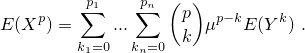
Transformation from central into raw

In this case, set argument type = 'raw'. Then function transformMoment returns

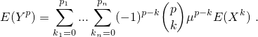
Transformation from raw to central

In this case, set argument type = 'central'. Then function transformMoment returns

Class momentList

The function transformMoment needs as input an S3-object of the class momentList which contains all known central and raw moments. It has four elements: The element centralMoments contains all known central moments of the distribution, where as rawMoments contains all raw moments of the distribution. Both are stored as a list. The elements centralMomentOrders and rawMomentOrders contain the corresponding orders of the moments. They are stored as a matrix or data.frame, each row represents one order of the moment. The number of columns of these matrices should be equal to the dimension of the distribution.

The function returns an object of class momentList which is expanded and includes the wanted moment and all moments that were computed during the calculation process.

Example

Calculate the raw moment (E(X_1X_2X_3^2)) for a three-dimensional random variable (X):

mList <- momentList(rawMomentOrders = diag(3),
                    rawMoments = list("m1", "m2", "m3"),
                    centralMomentOrders = expand.grid(list(0:1,0:1,0:2)),
                    centralMoments = as.list(c(1, 0, 0, "a", 0, letters[2:8])))

mList <- transformMoment(order = c(1,1,2), type = 'raw', 
                         momentList = mList, simplify = TRUE)

mList$rawMomentOrders
#>   [,1] [,2] [,3]
#>      0    0    0
#>      1    0    0
#>      0    1    0
#>      0    0    1
#> p    1    1    2

mList$rawMoments
#> [[1]]
#> [1] 1
#> 
#> [[2]]
#> [1] "m1"
#> 
#> [[3]]
#> [1] "m2"
#> 
#> [[4]]
#> [1] "m3"
#> 
#> [[5]]
#> g * m1 + h + m2 * (e * m1 + f) + m3 * (2 * (b * m2) + 2 * (c * 
#>     m1) + 2 * d + m3 * (a + m1 * m2))

The BEGG distribution

The bimodal extension of the generalized Gamma-Distribution (BEGG) was first introduced in

• Bulut, Y. M., & Arslan, O. (2015). A bimodal extension of the generalized gamma distribution. Revista Colombiana de Estadística, 38(2), 371-384.

It is a scale mixture of the generalized gamma distribution. The BEGG distribution is almost always bimodal. The two modes can have different shapes, depending on the parameters (α), (β), (δ_0), (δ_1), (η), (\epsilon), (μ) and (σ).

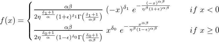
The density function can be calculated with dBEGG and is given by

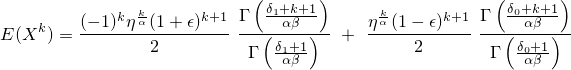
The k-th raw moment can be calculated with mBEGG and is given by

The density function can have very different shapes:

Testing if a distribution is unimodal

The function is.unimoal checks if an (unknown) distribution with compact support can be unimodal. It uses several inequalities that were introduced in

• Teuscher, F., & Guiard, V. (1995). Sharp inequalities between skewness and kurtosis for unimodal distributions. Statistics & probability letters, 22(3), 257-260.
• Johnson, N. L., & Rogers, C. A. (1951). The moment problem for unimodal distributions. The Annals of Mathematical Statistics, 433-439.
• Simpson, J. A., & Welch, B. L. (1960). Table of the bounds of the probability integral when the first four moments are given. Biometrika, 47(3/4), 399-410.

Depending on the inequality, moments up to order 2 or 4 are required. A distribution that satisfies all inequalities that contain only moments up to order 2 is called 2-b-unimodal. A distribution that satisfies all inequalities that contain only moments up to order 4 is called 4-b-unimodal. It is possible that a multimodal distribution satisfies all inequalities and is therefore 2- and even 4-bimodal. But if at least one of the inequalities is not satisfied, the distribution cannot be unimodal. In this case, the test returns not unimodal as the result.

Here are some examples using the BEGG distribution:

# example 1 (bimodal)
example1 <- mBEGG(order = 1:4, alpha = 2, beta = 2, delta0 = 1, delta1 = 4, eta = 1, eps = 0)
is.unimodal(-2, 2, example1)
#> [1] "not unimodal"

# example 2 (bimodal)
example2 <- mBEGG(order = 1:4, alpha = 2, beta = 1, delta0 = 0, delta1 = 2, eta = 1, eps = -0.5)
is.unimodal(-2, 3, example2)
#> [1] "4-b-unimodal"

# example 3 (bimodal)
example3 <- mBEGG(order = 1:4, alpha = 3, beta = 2, delta0 = 4, delta1 = 2, eta = 2, eps = 0.3)
is.unimodal(-2.5, 1.5, example3[1:2]) # test with moments of order 1 and 2
#> [1] "2-b-unimodal"
is.unimodal(-2.5, 1.5, example3) # test with moments of order 1 - 4
#> [1] "not unimodal"

# example 4 (unimodal)
example4 <- mBEGG(order = 1:4, alpha = 2, beta = 1, delta0 = 0, delta1 = 0, eta = 1, eps = 0.7)
is.unimodal(-4, 2, example4)
#> [1] "4-b-unimodal"

License

The function dtrunc of the package momcalc is a modified version of the function dtrunc of the package truncdist. Both packages are free open source software licensed under the GNU Public License (GPL 2.0 or above). The software is provided as is and comes WITHOUT WARRANTY.

CharlotteJana/momcalc documentation built on Oct. 17, 2019, 7:21 a.m.