README.md

In ChubingZeng/classo: Regularized Regression with Differential Penalties Integrating External Information

xtune: Tuning differential shrinkage parameters of penalized regression models based on external information

📗 Introduction

Motivation

In standard Lasso and Ridge regression, a single penalty parameter λ applied equally to all regression coefficients to control the amount of regularization in the model.

Better prediction accuracy may be achieved by allowing a differential amount of shrinkage. Ideally, we want to give a small penalty to important features and a large penalty to unimportant features. We guide the penalized regression model with external data Z that are potentially informative for the importance/effect size of coefficients and allow differential shrinkage modeled as a log-linear function of the external data.

The objective function of differential-shrinkage Lasso integrating external information is:

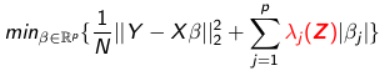
The objective function of differential-shrinkage Lasso integrating external information is:

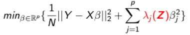
The idea of external data is that it provides us information on the importance/effect size of regression coefficients. It could be any nominal or quantitative feature-specific information, such as the grouping of predictors, prior knowledge of biological importance, external p-values, function annotations, etc. Each column of Z is a variable for features in design matrix X. Z is of dimension, where p is the number of features and q is the number of variables in Z.

Tuning multiple penalty parameters

Penalized regression fitting consists of two phases: (1) learning the tuning parameter(s) (2) estimating the regression coefficients giving the tuning parameter(s). Phase (1) is the key to achieve good performance. Cross-validation is widely used to tune a single penalty parameter, but it is computationally infeasible to tune more than three penalty parameters. We propose an Empirical Bayes approach to learn the multiple tuning parameters. The individual penalties are interpreted as variance terms of the priors (double exponential prior for Lasso and Gaussian prior for Ridge) in a random effect formulation of penalized regressions. A majorization-minimization algorithm is employed for implementation. Once the tuning parameters λs are estimated, and therefore the penalties are known, phase (2) - estimating the regression coefficients is done using glmnet.

Data structure examples

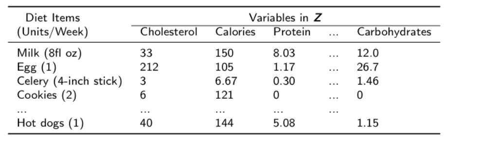
Suppose we want to predict a person's weight loss using his/her weekly dietary intake. Our external information Z could incorporate information about the levels of relevant food constituents in the dietary items.

Primary data X and Y: predicting an individual's weight loss by his/her weekly dietary items intake

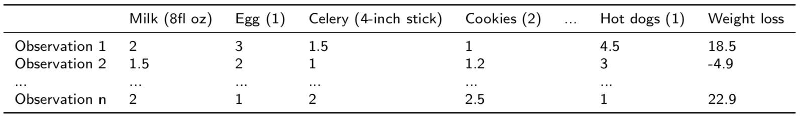
External information Z: the nutrition facts about each dietary item

📙 Installation

xtune can be installed from Github using the following command:

# install.packages("devtools")

library(devtools)
devtools::install_github("ChubingZeng/xtune")

library(xtune)

📘 Examples

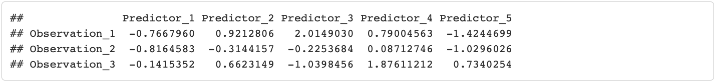
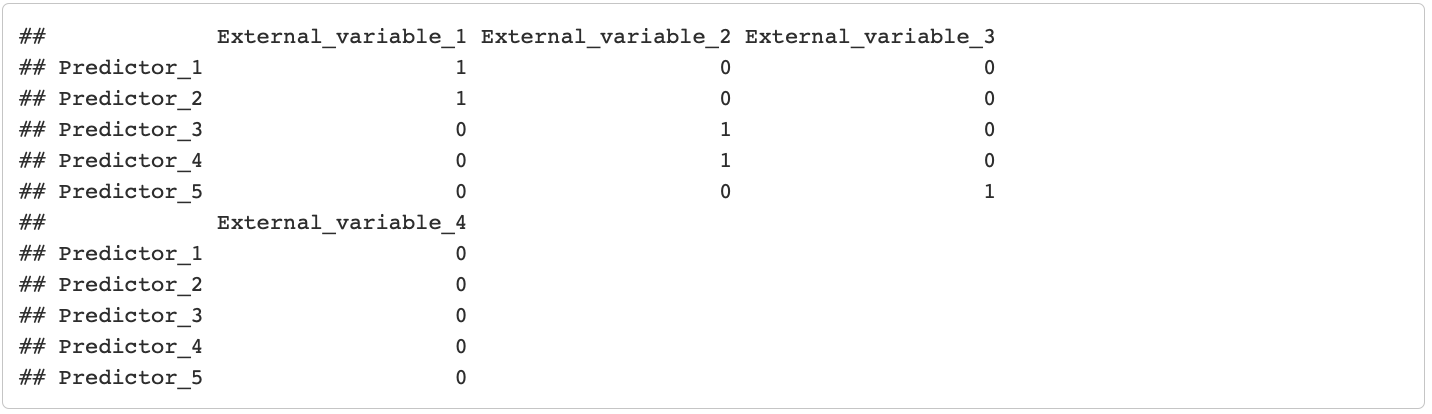
To show some examples on how to use this package, we simulated an example of data that contains 100 observations, 200 predictors, and a continuous outcome. The external information Z contains 4 columns, each column is indicator variable (can be viewed as the grouping of predictors).

## load the example data
data(example)

The data looks like:

example$X[1:3,1:5]

example$Z[1:5,]

xtune() is the core function to fit the integrated penalized regression model. At a minimum, you need to specify the predictor matrix X, outcome variable Y. If an external information matrix Z is provided, the function will incorporate Z to allow differential shrinkage based on Z. The estimated tuning parameters are returned in $penalty.vector.

If you do not provide external information Z, the function will perform empirical Bayes tuning to choose the single penalty parameter in penalized regression, as an alternative to cross-validation. You could compare the tuning parameter chosen by empirical Bayes tuning to that choose by cross-validation (see also cv.glmnet). The default penalty applied to the predictors is the Lasso penalty.

If you provide an identify matrix as external information Z to xtune(), the function will estimate a separate tuning parameter for each regression coefficient .

xtune.fit <- xtune(example$X,example$Y,example$Z)

## for ridge
## xtune.fit <- xtune(example$X,example$Y,example$Z,method = "ridge")

To view the penalty parameters estimated by xtune()

xtune.fit$penalty.vectors

The coef and predict functions can be used to extract beta coefficient estimates and predict response on new data.

coef(xtune.fit)
predict(xtune.fit, example$X)

Two real-world examples are also described in the vignettes to further illustrate the usage and syntax of this package.

ChubingZeng/classo documentation built on June 4, 2019, 12:37 p.m.