Vignette.md
In JVAdams/artiFISHal: A Pelagic Fish Community Simulator
artiFISHal Vignette
The following is an example using the
functions in the artiFISHal package. See README.md
for instructions on installing the package.
Start by loading the package.
library(artiFISHal)
===
Simulate a Population of Fish
Create a data frame with 18 columns in which each row describes a sub-population of fish to be placed in the artificial lake.
The first 11 columns must be completely filled in (no missing values).
- G = character, a one-letter nickname for the group (e.g., fish species and life stage) used in plotting
- Z = numeric, mean length (in mm)
- ZE = numeric, error around mean length, expressed as SD/mean
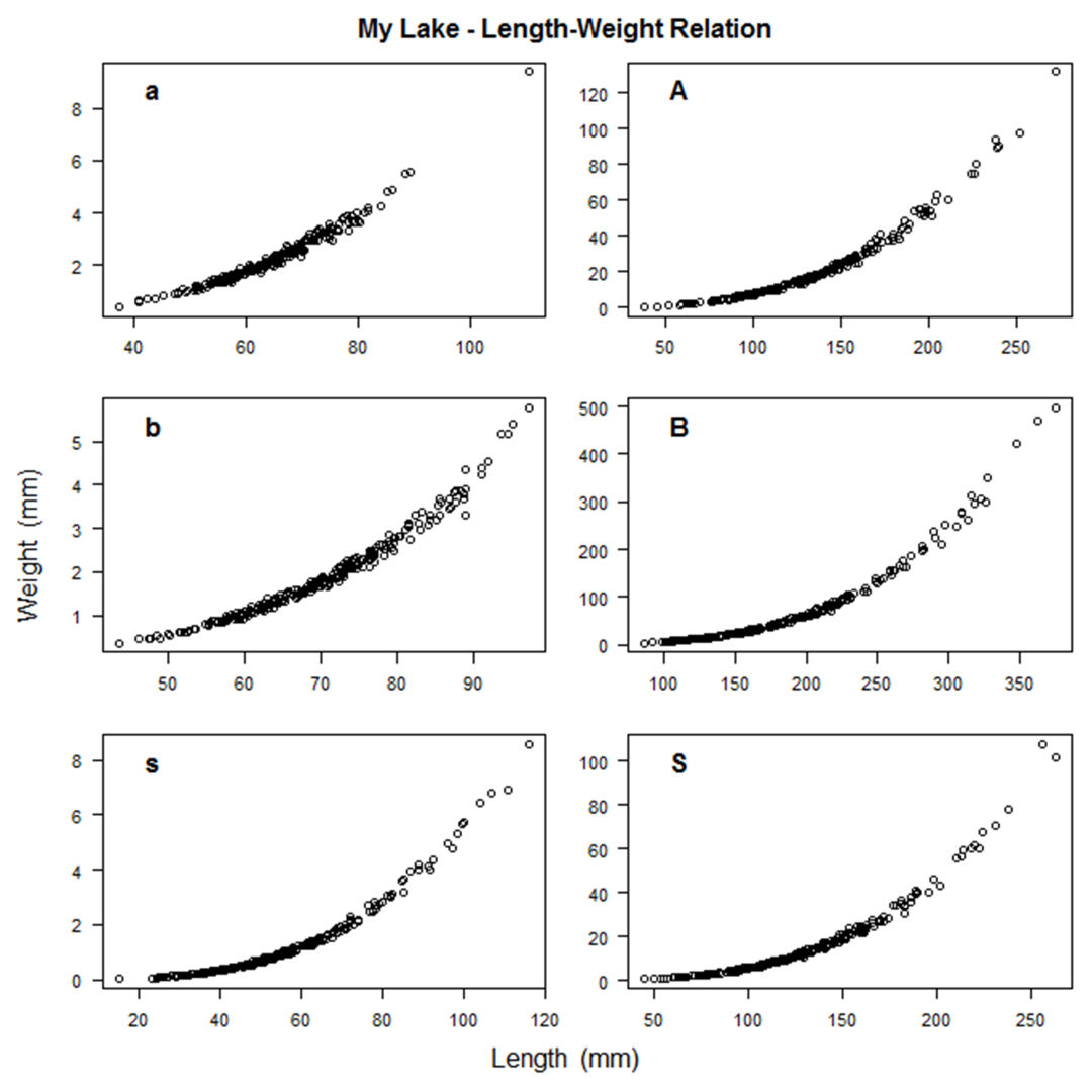
- LWC1, LWC2 = numeric, length-weight regression coefficients, where wt = LWC1*len^LWC2, (wt in g, len in mm)
- LWCE = numeric, error around weight estimate, expressed as SD(estimate)/estimate
- TSC1, TSC2 = numeric, target strength and length relation coefficients, ts = TSC1 + TSC2*log10(len/10), (ts in db, len in mm)
- TSCE = numeric, error around target strength estimate, expressed as SD(estimate)/estimate
- PropN = numeric, approximate proportion of population that the row represents (automatically adjusted to ensure they sum to 1)
The last 8 columns may have some missing values.
However, in each row, either water depth (WD and WDE) or distance to bottom (D2B and D2BE) must be filled in, but not both.
- E = numeric, mean easting (m)
- EE = numeric, error around easting, expressed as SD/mean
- N = numeric, mean northing (m)
- NE = numeric, error around northing, expressed as SD/mean
- WD = numeric, mean water depth (m)
- WDE = numeric, error around water depth, expressed as SD/mean
- D2B = numeric, mean distance to bottom (m)
- D2BE = numeric, error around distance to bottom, expressed as SD/mean
You may find that the easiest way to create this data frame is by entering the information in an external file,
e.g., a comma delimited file. In that case, you would read in the data frame using the read.csv function.
The data frame should be all character and numeric variables, so if you use read.csv, you should specify as.is=TRUE.
ExInputs <- read.csv("C:/temp/ExInputs.csv", as.is=TRUE)
For the purposes of this vignette, I will create the data frame using code.
ExInputs <- data.frame(
    Description = c("alewife small", "alewife small", "alewife large", "alewife large",
        "alewife large", "alewife large", "rainbow smelt small", "rainbow smelt small", "rainbow smelt large",
        "rainbow smelt large", "bloater small", "bloater small", "bloater large", "bloater large"),
    G = c("a", "a", "A", "A", "A", "A", "s", "s", "S", "S", "b", "b", "B", "B"),
    Z = c(65, 65, 127, 127, 127, 127, 55, 55, 127, 127, 70, 70, 190, 190),
    ZE = c(0.15, 0.15, 0.3, 0.3, 0.3, 0.3, 0.3, 0.3, 0.3, 0.3, 0.15, 0.15, 0.3, 0.3),
    LWC1 = 1e-8*c(1400, 1400, 1400, 1400, 1400, 1400, 481, 481, 481, 481, 102, 102, 102, 102),
    LWC2 = c(2.8638, 2.8638, 2.8638, 2.8638, 2.8638, 2.8638, 3.0331, 3.0331, 3.0331, 3.0331, 3.3812, 3.3812, 3.3812, 3.3812),
    LWCE = c(0.05, 0.05, 0.05, 0.05, 0.05, 0.05, 0.05, 0.05, 0.05, 0.05, 0.05, 0.05, 0.05, 0.05),
    TSC1 = c(-64.2, -64.2, -64.2, -64.2, -64.2, -64.2, -67.8, -67.8, -67.8, -67.8, -70.88, -70.88, -70.88, -70.88),
    TSC2 = c(20.5, 20.5, 20.5, 20.5, 20.5, 20.5, 19.9, 19.9, 19.9, 19.9, 25.54, 25.54, 25.54, 25.54),
    TSCE = c(0.03, 0.03, 0.05, 0.05, 0.05, 0.05, 0.05, 0.05, 0.08, 0.08, 0.03, 0.03, 0.04, 0.04),
    PropN = c(0.3, 0.3, 0.035, 0.035, 0.015, 0.015, 0.0375, 0.0375, 0.0375, 0.0375, 0.0375, 0.0375, 0.0375, 0.0375),
    E = 100*c(93, 170, 6, 289, 90, 179, 93, 170, 6, 289, 93, 170, 34, 233),
    EE = c(0.7, 0.4, 2.5, 0.1, 0.9, 0.6, 0.7, 0.4, 2.2, 0.1, 0.7, 0.4, 0.3, 0.1),
    N = 100*c(100, 100, 100, 100, 100, 100, 100, 100, 170, 170, 100, 100, 75, 75),
    NE = c(1, 1, 1, 1, 1, 1, 1, 1, 0.1, 0.1, 1, 1, 0.5, 0.5),
    WD = c(14, 14, 11, 11, 11, 11, 16, 16, 29, 29, 20, 20, NA, NA),
    WDE = c(0.2, 0.2, 0.2, 0.2, 0.2, 0.2, 0.2, 0.2, 0.3, 0.3, 0.2, 0.2, NA, NA),
    D2B = c(NA, NA, NA, NA, NA, NA, NA, NA, NA, NA, NA, NA, 15, 15),
    D2BE = c(NA, NA, NA, NA, NA, NA, NA, NA, NA, NA, NA, NA, 0.3, 0.3))
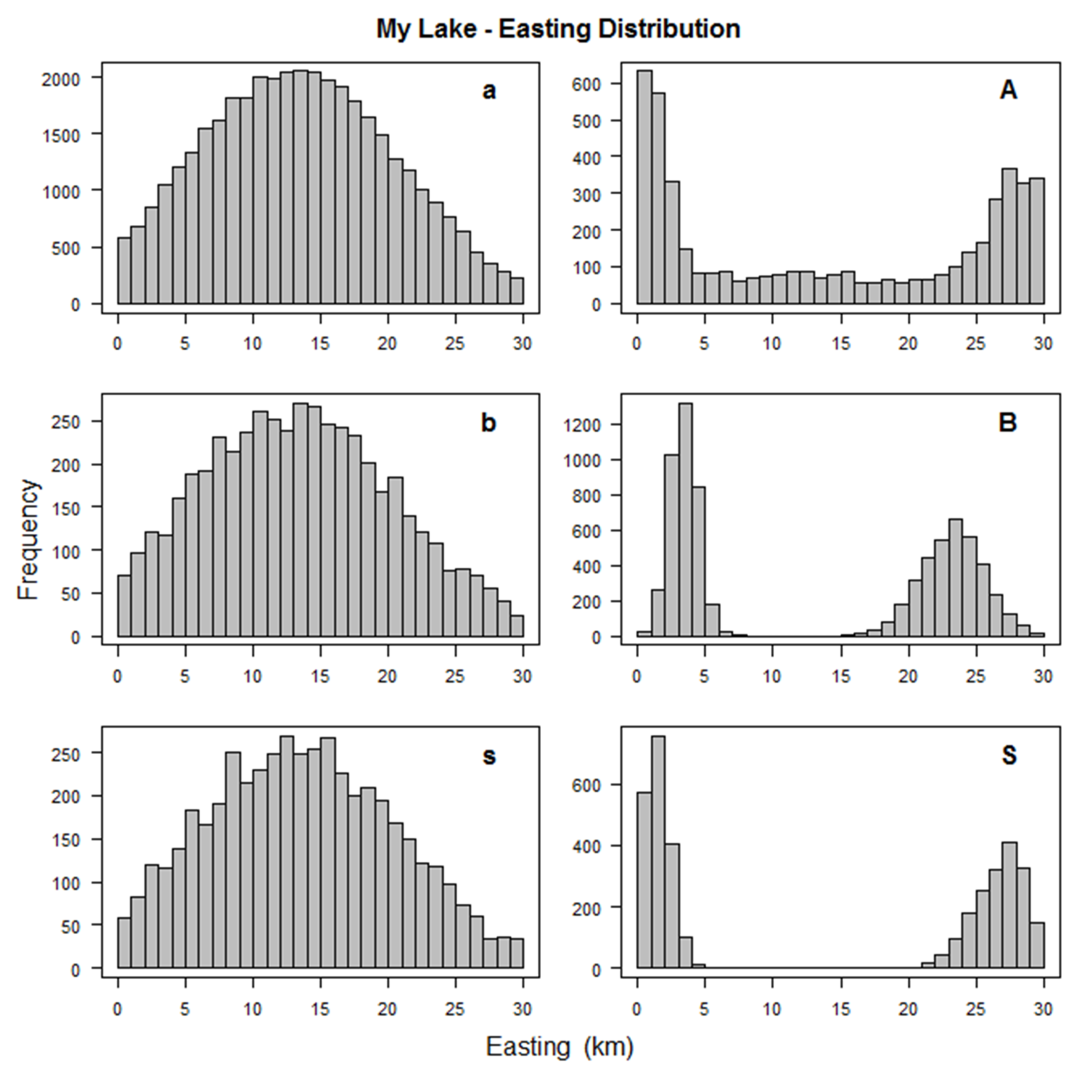
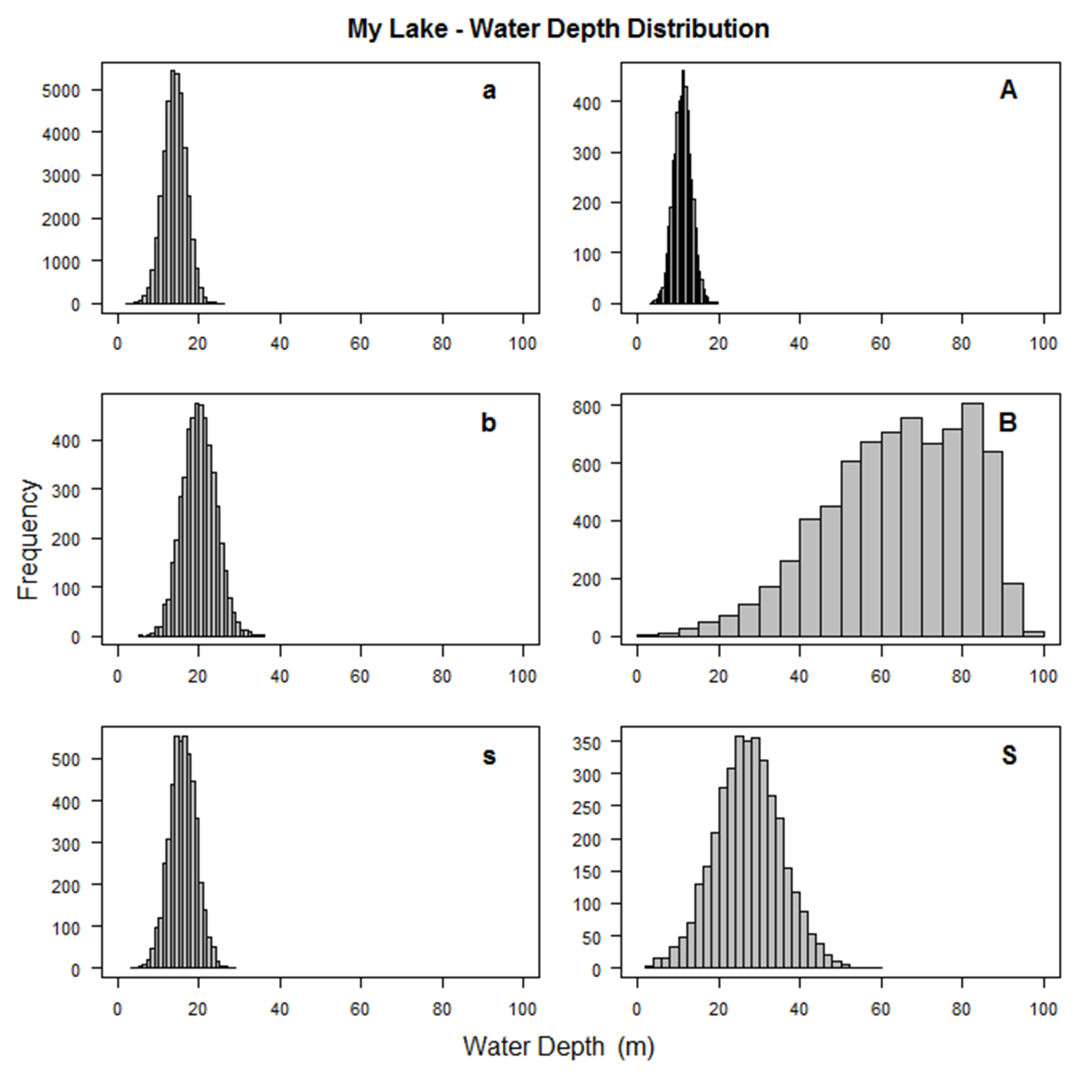
This data frame contains information on six groups of fish in 14 rows of data.
To get some idea of how this works, have a look at rows 3-6 which includes specifications for group A, alewife large.
The sizes of the fish (Z, ZE, LWC1, LWC3, LWCE, TSC1, TSC2, and TSCE) being simulated are the same in all four rows.
But, the locations of the fish are different: 3.5% are at easting 600 (with SD 2.5 * 600), 1.5% are at easting 9,000 (SD 0.9 * 9,000),
1.5% are at easting 17,900 (with SD 0.6 * 17,900), and 3.5% are at easting 28,900 (SD 0.1 * 28,900).
All of the groups of fish are located using water depth (WD and WDE), except for group B, bloater large,
which are located using distance to bottom (D2B and D2BE).
           Description G   Z   ZE       LWC1   LWC2 LWCE   TSC1  TSC2 TSCE  PropN     E  EE     N  NE WD WDE D2B D2BE
1        alewife small a  65 0.15 0.00001400 2.8638 0.05 -64.20 20.50 0.03 0.3000  9300 0.7 10000 1.0 14 0.2  NA   NA
2        alewife small a  65 0.15 0.00001400 2.8638 0.05 -64.20 20.50 0.03 0.3000 17000 0.4 10000 1.0 14 0.2  NA   NA
3        alewife large A 127 0.30 0.00001400 2.8638 0.05 -64.20 20.50 0.05 0.0350   600 2.5 10000 1.0 11 0.2  NA   NA
4        alewife large A 127 0.30 0.00001400 2.8638 0.05 -64.20 20.50 0.05 0.0350 28900 0.1 10000 1.0 11 0.2  NA   NA
5        alewife large A 127 0.30 0.00001400 2.8638 0.05 -64.20 20.50 0.05 0.0150  9000 0.9 10000 1.0 11 0.2  NA   NA
6        alewife large A 127 0.30 0.00001400 2.8638 0.05 -64.20 20.50 0.05 0.0150 17900 0.6 10000 1.0 11 0.2  NA   NA
7  rainbow smelt small s  55 0.30 0.00000481 3.0331 0.05 -67.80 19.90 0.05 0.0375  9300 0.7 10000 1.0 16 0.2  NA   NA
8  rainbow smelt small s  55 0.30 0.00000481 3.0331 0.05 -67.80 19.90 0.05 0.0375 17000 0.4 10000 1.0 16 0.2  NA   NA
9  rainbow smelt large S 127 0.30 0.00000481 3.0331 0.05 -67.80 19.90 0.08 0.0375   600 2.2 17000 0.1 29 0.3  NA   NA
10 rainbow smelt large S 127 0.30 0.00000481 3.0331 0.05 -67.80 19.90 0.08 0.0375 28900 0.1 17000 0.1 29 0.3  NA   NA
11       bloater small b  70 0.15 0.00000102 3.3812 0.05 -70.88 25.54 0.03 0.0375  9300 0.7 10000 1.0 20 0.2  NA   NA
12       bloater small b  70 0.15 0.00000102 3.3812 0.05 -70.88 25.54 0.03 0.0375 17000 0.4 10000 1.0 20 0.2  NA   NA
13       bloater large B 190 0.30 0.00000102 3.3812 0.05 -70.88 25.54 0.04 0.0375  3400 0.3  7500 0.5 NA  NA  15  0.3
14       bloater large B 190 0.30 0.00000102 3.3812 0.05 -70.88 25.54 0.04 0.0375 23300 0.1  7500 0.5 NA  NA  15  0.3
Now you can use the SimFish function to simulate the fish population based on these parameters.
myfish <- SimFish(LakeName="My Lake", LkWidth=30000, LkLength=20000, BotDepMin=20, BotDepMax=100,
    FishParam=ExInputs, TotNFish=100000, Seed=545)
Look at the true total number and weight of each fish group in the population.
myfish$Truth

          n         kg     nperha       kgperha
a     38521  88.639197 0.64201667 0.00147731995
A      4791  88.455773 0.07985000 0.00147426288
b      4896   9.576029 0.08160000 0.00015960048
B      7328 527.063943 0.12213333 0.00878439905
s      4756   5.584219 0.07926667 0.00009307032
S      3648  54.411041 0.06080000 0.00090685069
Total 63940 773.730202 1.06566667 0.01289550337
Look at the fish population that you just simulated. Each row represents a single individual fish.
Columns describe the group, location, and size of the fish.
head(myfish$Fish)

  G    f.east   f.north    f.d2sh  f.botdep   f.wdep  f.d2bot      len       wt        ts
1 a 12355.212 16823.528 13466.323 100.00000 13.60617 86.39383 59.81102 1.595275 -49.49159
2 a 12559.997 12749.377 13671.108 100.00000 12.48335 87.51665 64.93574 2.106270 -44.95919
3 a  4237.675 14277.050  5348.786  96.27815 20.25294 76.02521 80.84223 4.227741 -46.51572
4 a  2185.455  5228.477  3296.566  59.33820 16.64036 42.69784 52.59334 1.191047 -48.87585
5 a  4965.597 17912.420  6076.708 100.00000 12.44079 87.55921 78.76110 3.766953 -46.85894
9 a  9106.080 16052.540 10217.191 100.00000 12.18392 87.81608 64.67095 2.049004 -48.81689
Simulating a fish population that looks the way you intended may take some trial and error.
A number of graphs are created illustrating the fish population that you've simulated to aid in this trial and error process.
A few examples are shown below.
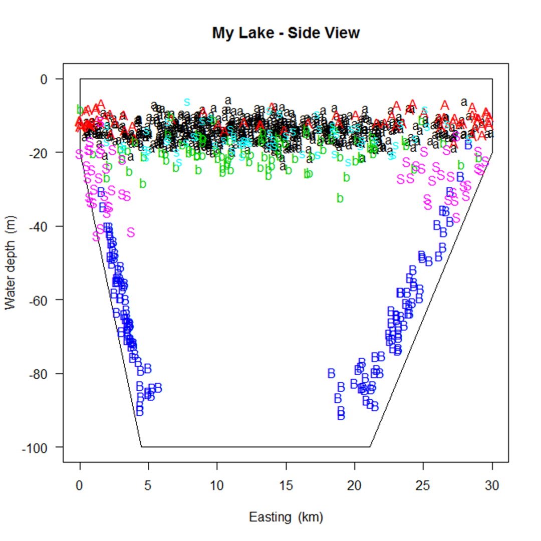
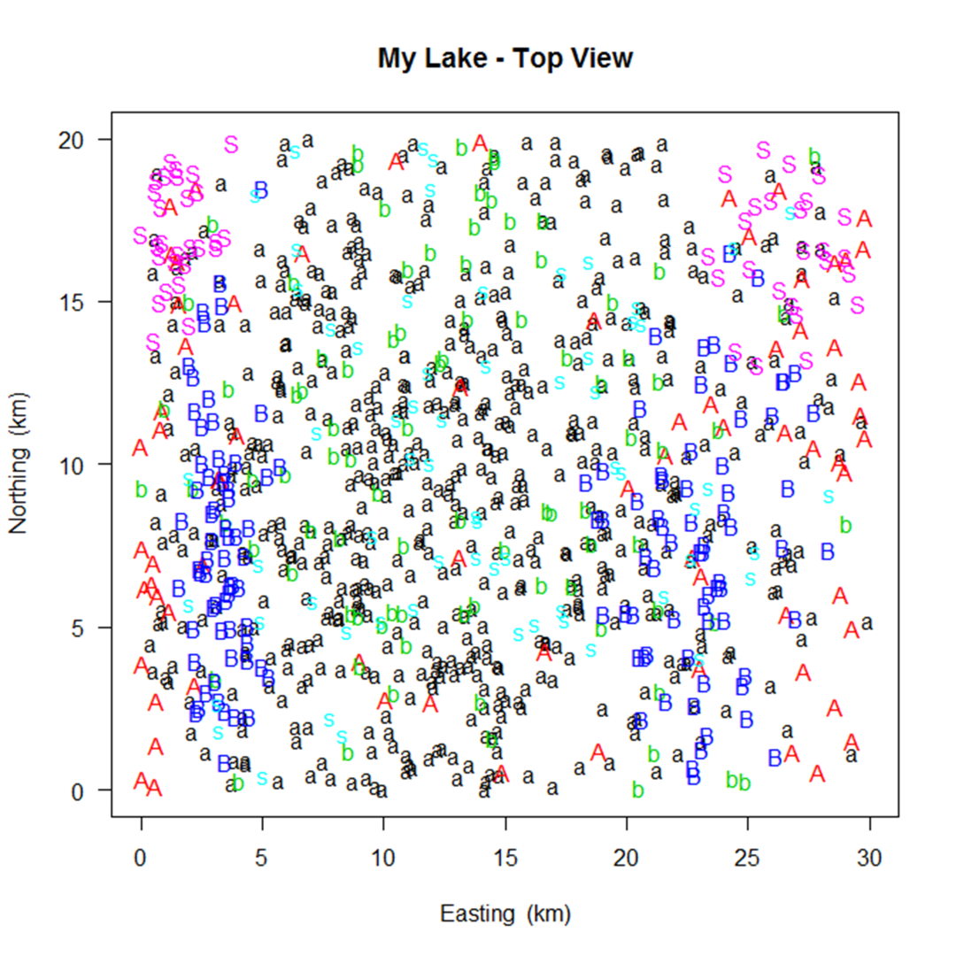
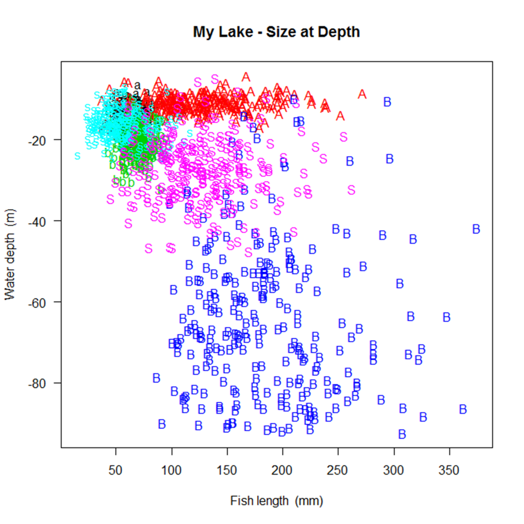
In the process of creating the population, SimFish will eliminate fish based on their size
(length or weight less than zero or target strength outside the allowable range) or
location (easting, northing, water depth, bottom depth, or distance to shore outside their allowable ranges).
You will likely end up with fewer fish than you requested.
But, if you end up with far fewer fish than expected, you should look at the proportion of fish excluded
to troubleshoot where in the inputs the problem might lie.
myfish$PropExcluded

LengthWeight           TS      Easting     Northing   WaterDepth  BottomDepth      D2Shore
     0.00000      0.00020      0.09728      0.27628      0.09472      0.04808      0.08345
The output from SimFish also keeps the inputs that were supplied as arguments for use in later sampling and summarization.
myfish$LakeInfo

$LakeName
[1] "My Lake"

$LkWidth
[1] 30000

$LkLength
[1] 20000

$BotDepMin
[1] 20

$BotDepMax
[1] 100

$BotDepVertex
[1] 200

$ints
[1]  20 290

$slopes
[1]  0.018 -0.009

$d2shr.we
[1] 1111.111 2222.222


myfish$FishInfo

$TotNFish
[1] 100000

$TSRange
[1] -65 -20

$Seed
[1] 545


head(myfish$FishParam)

    Description G   Z   ZE     LWC1   LWC2 LWCE  TSC1 TSC2 TSCE PropN     E  EE     N NE WD WDE D2B D2BE Nfish
1 alewife small a  65 0.15 0.000014 2.8638 0.05 -64.2 20.5 0.03 0.300  9300 0.7 10000  1 14 0.2  NA   NA 30000
2 alewife small a  65 0.15 0.000014 2.8638 0.05 -64.2 20.5 0.03 0.300 17000 0.4 10000  1 14 0.2  NA   NA 30000
3 alewife large A 127 0.30 0.000014 2.8638 0.05 -64.2 20.5 0.05 0.035   600 2.5 10000  1 11 0.2  NA   NA  3500
4 alewife large A 127 0.30 0.000014 2.8638 0.05 -64.2 20.5 0.05 0.035 28900 0.1 10000  1 11 0.2  NA   NA  3500
5 alewife large A 127 0.30 0.000014 2.8638 0.05 -64.2 20.5 0.05 0.015  9000 0.9 10000  1 11 0.2  NA   NA  1500
6 alewife large A 127 0.30 0.000014 2.8638 0.05 -64.2 20.5 0.05 0.015 17900 0.6 10000  1 11 0.2  NA   NA  1500
===
Sample the Fish Population
Once you have the population the way you want it, you can sample the population with a virtual acoustic and midwater trawl survey.
mysurv <- SampFish(SimPop=myfish, NumEvents=10, AcNum=15, AcInterval=30000, AcLayer=10, AcAngle=7,
    MtNum=30, MtHt=10, MtWd=10, MtLen=2000, Seed=341)
This will display the following output,
Mean number of fish per acoustic transect = 8
Mean number of fish per midwater trawl tow = 2.6
in addition to a few graphs summarizing the catch. The output from SampFish has two sample data frames,
one for the acoustic targets detected and one for the midwater trawl catch.
head(mysurv$Targets)

    Event ACid  ACnorth interval layer    f.east  f.north    f.d2sh  f.botdep   f.wdep  f.d2bot        ts G      len       wt
1       1    1 226.4871    15000    15  4731.921 226.1967  5843.032 100.00000 12.35791 87.64209 -46.21903 a 75.13432 3.153108
1.1     1    1 226.4871    15000    15 10068.349 226.3635 11179.460 100.00000 14.20916 85.79084 -49.27524 a 55.91032 1.434534
1.2     1    1 226.4871    15000    15 17416.707 226.2335 14805.515 100.00000 13.54249 86.45751 -50.01943 a 72.71979 2.738727
1.3     1    1 226.4871    15000    15 17533.835 226.6315 14688.387 100.00000 11.54177 88.45823 -50.25154 a 65.08561 2.201175
1.4     1    1 226.4871    15000    15  1348.329 226.4841  2459.440  44.26992 12.48686 31.78306 -46.93286 A 72.70365 3.034980
1.5     1    1 226.4871    15000    15 27787.635 226.7050  4434.588  39.91129 10.41862 29.49267 -45.91410 A 67.37459 2.504339


head(mysurv$MtCatch)

     Event ACid ACnorth MTRid  MTReast   MTRd2sh   MTRbdep   MTRwdep MTRd2bot G       len         wt   f.east  f.north    f.d2sh  f.botdep    f.wdep  f.d2bot        ts
55       1    5 5559.82    55 9985.163 11096.274 100.00000 18.909694 81.09031 s  42.33906  0.4159183 9040.986 5559.049 10152.098 100.00000 16.809346 83.19065 -58.54070
55.1     1    5 5559.82    55 9985.163 11096.274 100.00000 18.909694 81.09031 b  53.75177  0.7422804 9891.081 5562.400 11002.192 100.00000 19.031482 80.96852 -51.00658
58       1    5 5559.82    58 2135.943  3247.054  58.44697 17.542449 40.90452 a  55.44073  1.4194104 2616.979 5558.572  3728.090  67.10562 16.214844 50.89077 -50.63201
58.1     1    5 5559.82    58 2135.943  3247.054  58.44697 17.542449 40.90452 a  81.21204  4.2189988 2413.535 5562.214  3524.646  63.44363 14.960325 48.48330 -41.96773
58.2     1    5 5559.82    58 2135.943  3247.054  58.44697 17.542449 40.90452 a  67.05389  2.4610922 2518.213 5564.127  3629.325  65.32784 14.721495 50.60635 -46.39444
87       1    8 9559.82    87 2474.812  3585.923  64.54662  8.915031 55.63159 A 122.05264 14.9580374 3229.151 9558.463  4340.262  78.12471  9.861536 68.26318 -42.00870
The output from SampFish also keeps the inputs supplied as arguments for use in later sampling and summarization.
mysurv$SurvParam

 NumEvents      AcNum AcInterval    AcLayer    AcAngle      MtNum       MtHt       MtWd      MtLen   MtMinCat    MtMulti       Seed
        10         15      30000         10          7         30         10         10       2000          2          6        341
===
Generate Estimates from the Sample
Estimate the number and biomass of fish per unit area sampled using the AcMtEst function
which combines the acoustic and midwater trawl data.
perf <- AcMtEst(SimPop=myfish, AcMtSurv=mysurv, Seed=927)
head(perf)

  Event G     nperha       kgperha
1     1 a 0.02927073 0.00008536381
2     1 A 0.02697084 0.00022705222
3     1 b 0.01429321 0.00001932634
4     1 B 0.00000000 0.00000000000
5     1 s 0.01429321 0.00002859123
6     1 S 0.00000000 0.00000000000
The virtual acoustic and midwater trawl surveys carried out by SampFish are assumed to be perfect with no issues of fish availability,
acoustic dead zones, or trawl selectivity.
If you wish to introduce availability or selectivity functions, you may do so in the AcMtEst function.
For the target data, fish are excluded from the sample if they are located in zones unavailable to the acoustic transducer
specified with the argument AcExcl.
For the catch data, fish are excluded from the sample if they are located in zones unavailable to the midwater trawl
specified with the argument MtExcl.
In addition, selectivity curves can be specified for different panels of the midwater trawl using the arguments
PanelProps and SelecParam.
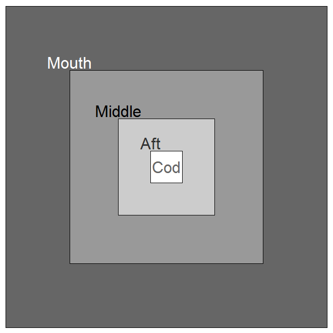
The PanelProps argument is used to denote the relative sizes of four different panels in the trawl,
from the mouth (outermost panel) to the cod end (innermost panel).
You can get a fish's-eye view of the panel sizes denoted using the ViewZones function.
ViewZones(PanelProp = c(0.4, 0.3, 0.2, 0.1))
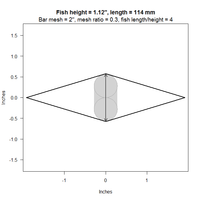
The SelecParam argument is used to denote the mesh selectivity for each fish group (species, life stage) and trawl panel zone.
You can use the MeshPass function to determine the largest height (or depth) of a fish that can pass through a
single diamond-shaped mesh of a net, provided the size of the mesh BarMesh,
the height to width ratio of the mesh H2WRatio,
and the length to height ratio of the fish L2HRatio.
MeshPass(BarMesh=2, H2WRatio=0.3, L2HRatio=4)
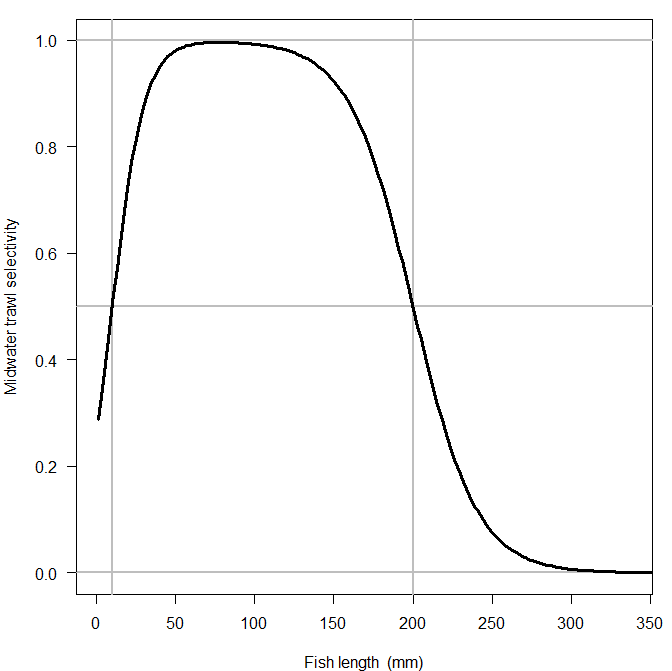
A double logistic regression function is used to specify selectivity as a function of fish total length
using two slopes and two inflection points.
If you have some notion of what the selectivity curve should look like,
you can use the TuneSelec function to discover the corresponding parameters using interactive sliders.
TuneSelec()
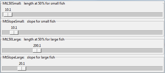
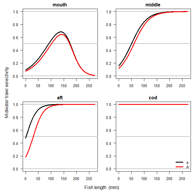
Once you have chosen the selectivity parameters you want to use, put them in a data frame.
selec <- data.frame(
    G = c("A", "a", "A", "a", "A", "a"),
    Zone = c("mouth", "mouth", "middle", "middle", "aft", "aft"),
    MtL50Small = c(100, 90, 60, 50, 30, 2),
    MtSlopeSmall = c(40, 40, 30, 30, 20, 20),
    MtL50Large = c(180, 180, Inf, Inf, Inf, Inf),
    MtSlopeLarge = c(20, 20, 100, 100, 100, 100))
selec

  G   Zone MtL50Small MtSlopeSmall MtL50Large MtSlopeLarge
1 A  mouth        100           40        180           20
2 a  mouth         90           40        180           20
3 A middle         60           30        Inf          100
4 a middle         50           30        Inf          100
5 A    aft         30           20        Inf          100
6 a    aft          2           20        Inf          100
Then you can visually compare the selectivity curves for the different fish groups using the ViewSelec function.
ViewSelec(selec)
If all looks well, you can now derive estimates from the survey, incorporating these availabilities and selectivities.
imperf <- AcMtEst(SimPop=myfish, AcMtSurv=mysurv, SelecParam=selec, AcExcl=c(5, 10), MtExcl=c(2, 2), Seed=204)
head(imperf)

  Event G     nperha       kgperha
1     1 a 0.04153298 0.00013806848
2     1 A 0.02768865 0.00020809515
3     1 b 0.00000000 0.00000000000
4     1 B 0.00000000 0.00000000000
5     1 s 0.01384433 0.00004962851
6     1 S 0.00000000 0.00000000000
JVAdams/artiFISHal documentation built on May 7, 2019, 10:14 a.m.
R Package Documentation
Browse R Packages
We want your feedback!
Note that we can't provide technical support on individual packages. You should contact the package authors for that.
artiFISHal Vignette
The following is an example using the functions in the artiFISHal package. See README.md for instructions on installing the package.
Start by loading the package.
library(artiFISHal)
===
Simulate a Population of Fish
Create a data frame with 18 columns in which each row describes a sub-population of fish to be placed in the artificial lake. The first 11 columns must be completely filled in (no missing values).
- G = character, a one-letter nickname for the group (e.g., fish species and life stage) used in plotting
- Z = numeric, mean length (in mm)
- ZE = numeric, error around mean length, expressed as SD/mean
- LWC1, LWC2 = numeric, length-weight regression coefficients, where wt = LWC1*len^LWC2, (wt in g, len in mm)
- LWCE = numeric, error around weight estimate, expressed as SD(estimate)/estimate
- TSC1, TSC2 = numeric, target strength and length relation coefficients, ts = TSC1 + TSC2*log10(len/10), (ts in db, len in mm)
- TSCE = numeric, error around target strength estimate, expressed as SD(estimate)/estimate
- PropN = numeric, approximate proportion of population that the row represents (automatically adjusted to ensure they sum to 1)
The last 8 columns may have some missing values. However, in each row, either water depth (WD and WDE) or distance to bottom (D2B and D2BE) must be filled in, but not both.
- E = numeric, mean easting (m)
- EE = numeric, error around easting, expressed as SD/mean
- N = numeric, mean northing (m)
- NE = numeric, error around northing, expressed as SD/mean
- WD = numeric, mean water depth (m)
- WDE = numeric, error around water depth, expressed as SD/mean
- D2B = numeric, mean distance to bottom (m)
- D2BE = numeric, error around distance to bottom, expressed as SD/mean
You may find that the easiest way to create this data frame is by entering the information in an external file,
e.g., a comma delimited file. In that case, you would read in the data frame using the read.csv function.
The data frame should be all character and numeric variables, so if you use read.csv, you should specify as.is=TRUE.
ExInputs <- read.csv("C:/temp/ExInputs.csv", as.is=TRUE)
For the purposes of this vignette, I will create the data frame using code.
ExInputs <- data.frame(
Description = c("alewife small", "alewife small", "alewife large", "alewife large",
"alewife large", "alewife large", "rainbow smelt small", "rainbow smelt small", "rainbow smelt large",
"rainbow smelt large", "bloater small", "bloater small", "bloater large", "bloater large"),
G = c("a", "a", "A", "A", "A", "A", "s", "s", "S", "S", "b", "b", "B", "B"),
Z = c(65, 65, 127, 127, 127, 127, 55, 55, 127, 127, 70, 70, 190, 190),
ZE = c(0.15, 0.15, 0.3, 0.3, 0.3, 0.3, 0.3, 0.3, 0.3, 0.3, 0.15, 0.15, 0.3, 0.3),
LWC1 = 1e-8*c(1400, 1400, 1400, 1400, 1400, 1400, 481, 481, 481, 481, 102, 102, 102, 102),
LWC2 = c(2.8638, 2.8638, 2.8638, 2.8638, 2.8638, 2.8638, 3.0331, 3.0331, 3.0331, 3.0331, 3.3812, 3.3812, 3.3812, 3.3812),
LWCE = c(0.05, 0.05, 0.05, 0.05, 0.05, 0.05, 0.05, 0.05, 0.05, 0.05, 0.05, 0.05, 0.05, 0.05),
TSC1 = c(-64.2, -64.2, -64.2, -64.2, -64.2, -64.2, -67.8, -67.8, -67.8, -67.8, -70.88, -70.88, -70.88, -70.88),
TSC2 = c(20.5, 20.5, 20.5, 20.5, 20.5, 20.5, 19.9, 19.9, 19.9, 19.9, 25.54, 25.54, 25.54, 25.54),
TSCE = c(0.03, 0.03, 0.05, 0.05, 0.05, 0.05, 0.05, 0.05, 0.08, 0.08, 0.03, 0.03, 0.04, 0.04),
PropN = c(0.3, 0.3, 0.035, 0.035, 0.015, 0.015, 0.0375, 0.0375, 0.0375, 0.0375, 0.0375, 0.0375, 0.0375, 0.0375),
E = 100*c(93, 170, 6, 289, 90, 179, 93, 170, 6, 289, 93, 170, 34, 233),
EE = c(0.7, 0.4, 2.5, 0.1, 0.9, 0.6, 0.7, 0.4, 2.2, 0.1, 0.7, 0.4, 0.3, 0.1),
N = 100*c(100, 100, 100, 100, 100, 100, 100, 100, 170, 170, 100, 100, 75, 75),
NE = c(1, 1, 1, 1, 1, 1, 1, 1, 0.1, 0.1, 1, 1, 0.5, 0.5),
WD = c(14, 14, 11, 11, 11, 11, 16, 16, 29, 29, 20, 20, NA, NA),
WDE = c(0.2, 0.2, 0.2, 0.2, 0.2, 0.2, 0.2, 0.2, 0.3, 0.3, 0.2, 0.2, NA, NA),
D2B = c(NA, NA, NA, NA, NA, NA, NA, NA, NA, NA, NA, NA, 15, 15),
D2BE = c(NA, NA, NA, NA, NA, NA, NA, NA, NA, NA, NA, NA, 0.3, 0.3))
This data frame contains information on six groups of fish in 14 rows of data.
To get some idea of how this works, have a look at rows 3-6 which includes specifications for group A, alewife large.
The sizes of the fish (Z, ZE, LWC1, LWC3, LWCE, TSC1, TSC2, and TSCE) being simulated are the same in all four rows.
But, the locations of the fish are different: 3.5% are at easting 600 (with SD 2.5 * 600), 1.5% are at easting 9,000 (SD 0.9 * 9,000),
1.5% are at easting 17,900 (with SD 0.6 * 17,900), and 3.5% are at easting 28,900 (SD 0.1 * 28,900).
All of the groups of fish are located using water depth (WD and WDE), except for group B, bloater large,
which are located using distance to bottom (D2B and D2BE).
Description G Z ZE LWC1 LWC2 LWCE TSC1 TSC2 TSCE PropN E EE N NE WD WDE D2B D2BE
1 alewife small a 65 0.15 0.00001400 2.8638 0.05 -64.20 20.50 0.03 0.3000 9300 0.7 10000 1.0 14 0.2 NA NA
2 alewife small a 65 0.15 0.00001400 2.8638 0.05 -64.20 20.50 0.03 0.3000 17000 0.4 10000 1.0 14 0.2 NA NA
3 alewife large A 127 0.30 0.00001400 2.8638 0.05 -64.20 20.50 0.05 0.0350 600 2.5 10000 1.0 11 0.2 NA NA
4 alewife large A 127 0.30 0.00001400 2.8638 0.05 -64.20 20.50 0.05 0.0350 28900 0.1 10000 1.0 11 0.2 NA NA
5 alewife large A 127 0.30 0.00001400 2.8638 0.05 -64.20 20.50 0.05 0.0150 9000 0.9 10000 1.0 11 0.2 NA NA
6 alewife large A 127 0.30 0.00001400 2.8638 0.05 -64.20 20.50 0.05 0.0150 17900 0.6 10000 1.0 11 0.2 NA NA
7 rainbow smelt small s 55 0.30 0.00000481 3.0331 0.05 -67.80 19.90 0.05 0.0375 9300 0.7 10000 1.0 16 0.2 NA NA
8 rainbow smelt small s 55 0.30 0.00000481 3.0331 0.05 -67.80 19.90 0.05 0.0375 17000 0.4 10000 1.0 16 0.2 NA NA
9 rainbow smelt large S 127 0.30 0.00000481 3.0331 0.05 -67.80 19.90 0.08 0.0375 600 2.2 17000 0.1 29 0.3 NA NA
10 rainbow smelt large S 127 0.30 0.00000481 3.0331 0.05 -67.80 19.90 0.08 0.0375 28900 0.1 17000 0.1 29 0.3 NA NA
11 bloater small b 70 0.15 0.00000102 3.3812 0.05 -70.88 25.54 0.03 0.0375 9300 0.7 10000 1.0 20 0.2 NA NA
12 bloater small b 70 0.15 0.00000102 3.3812 0.05 -70.88 25.54 0.03 0.0375 17000 0.4 10000 1.0 20 0.2 NA NA
13 bloater large B 190 0.30 0.00000102 3.3812 0.05 -70.88 25.54 0.04 0.0375 3400 0.3 7500 0.5 NA NA 15 0.3
14 bloater large B 190 0.30 0.00000102 3.3812 0.05 -70.88 25.54 0.04 0.0375 23300 0.1 7500 0.5 NA NA 15 0.3
Now you can use the SimFish function to simulate the fish population based on these parameters.
myfish <- SimFish(LakeName="My Lake", LkWidth=30000, LkLength=20000, BotDepMin=20, BotDepMax=100,
FishParam=ExInputs, TotNFish=100000, Seed=545)
Look at the true total number and weight of each fish group in the population.
myfish$Truth
n kg nperha kgperha
a 38521 88.639197 0.64201667 0.00147731995
A 4791 88.455773 0.07985000 0.00147426288
b 4896 9.576029 0.08160000 0.00015960048
B 7328 527.063943 0.12213333 0.00878439905
s 4756 5.584219 0.07926667 0.00009307032
S 3648 54.411041 0.06080000 0.00090685069
Total 63940 773.730202 1.06566667 0.01289550337
Look at the fish population that you just simulated. Each row represents a single individual fish. Columns describe the group, location, and size of the fish.
head(myfish$Fish)
G f.east f.north f.d2sh f.botdep f.wdep f.d2bot len wt ts
1 a 12355.212 16823.528 13466.323 100.00000 13.60617 86.39383 59.81102 1.595275 -49.49159
2 a 12559.997 12749.377 13671.108 100.00000 12.48335 87.51665 64.93574 2.106270 -44.95919
3 a 4237.675 14277.050 5348.786 96.27815 20.25294 76.02521 80.84223 4.227741 -46.51572
4 a 2185.455 5228.477 3296.566 59.33820 16.64036 42.69784 52.59334 1.191047 -48.87585
5 a 4965.597 17912.420 6076.708 100.00000 12.44079 87.55921 78.76110 3.766953 -46.85894
9 a 9106.080 16052.540 10217.191 100.00000 12.18392 87.81608 64.67095 2.049004 -48.81689
Simulating a fish population that looks the way you intended may take some trial and error. A number of graphs are created illustrating the fish population that you've simulated to aid in this trial and error process. A few examples are shown below.
In the process of creating the population, SimFish will eliminate fish based on their size
(length or weight less than zero or target strength outside the allowable range) or
location (easting, northing, water depth, bottom depth, or distance to shore outside their allowable ranges).
You will likely end up with fewer fish than you requested.
But, if you end up with far fewer fish than expected, you should look at the proportion of fish excluded
to troubleshoot where in the inputs the problem might lie.
myfish$PropExcluded
LengthWeight TS Easting Northing WaterDepth BottomDepth D2Shore
0.00000 0.00020 0.09728 0.27628 0.09472 0.04808 0.08345
The output from SimFish also keeps the inputs that were supplied as arguments for use in later sampling and summarization.
myfish$LakeInfo
$LakeName
[1] "My Lake"
$LkWidth
[1] 30000
$LkLength
[1] 20000
$BotDepMin
[1] 20
$BotDepMax
[1] 100
$BotDepVertex
[1] 200
$ints
[1] 20 290
$slopes
[1] 0.018 -0.009
$d2shr.we
[1] 1111.111 2222.222
myfish$FishInfo
$TotNFish
[1] 100000
$TSRange
[1] -65 -20
$Seed
[1] 545
head(myfish$FishParam)
Description G Z ZE LWC1 LWC2 LWCE TSC1 TSC2 TSCE PropN E EE N NE WD WDE D2B D2BE Nfish
1 alewife small a 65 0.15 0.000014 2.8638 0.05 -64.2 20.5 0.03 0.300 9300 0.7 10000 1 14 0.2 NA NA 30000
2 alewife small a 65 0.15 0.000014 2.8638 0.05 -64.2 20.5 0.03 0.300 17000 0.4 10000 1 14 0.2 NA NA 30000
3 alewife large A 127 0.30 0.000014 2.8638 0.05 -64.2 20.5 0.05 0.035 600 2.5 10000 1 11 0.2 NA NA 3500
4 alewife large A 127 0.30 0.000014 2.8638 0.05 -64.2 20.5 0.05 0.035 28900 0.1 10000 1 11 0.2 NA NA 3500
5 alewife large A 127 0.30 0.000014 2.8638 0.05 -64.2 20.5 0.05 0.015 9000 0.9 10000 1 11 0.2 NA NA 1500
6 alewife large A 127 0.30 0.000014 2.8638 0.05 -64.2 20.5 0.05 0.015 17900 0.6 10000 1 11 0.2 NA NA 1500
===
Sample the Fish Population
Once you have the population the way you want it, you can sample the population with a virtual acoustic and midwater trawl survey.
mysurv <- SampFish(SimPop=myfish, NumEvents=10, AcNum=15, AcInterval=30000, AcLayer=10, AcAngle=7,
MtNum=30, MtHt=10, MtWd=10, MtLen=2000, Seed=341)
This will display the following output,
Mean number of fish per acoustic transect = 8
Mean number of fish per midwater trawl tow = 2.6
in addition to a few graphs summarizing the catch. The output from SampFish has two sample data frames,
one for the acoustic targets detected and one for the midwater trawl catch.
head(mysurv$Targets)
Event ACid ACnorth interval layer f.east f.north f.d2sh f.botdep f.wdep f.d2bot ts G len wt
1 1 1 226.4871 15000 15 4731.921 226.1967 5843.032 100.00000 12.35791 87.64209 -46.21903 a 75.13432 3.153108
1.1 1 1 226.4871 15000 15 10068.349 226.3635 11179.460 100.00000 14.20916 85.79084 -49.27524 a 55.91032 1.434534
1.2 1 1 226.4871 15000 15 17416.707 226.2335 14805.515 100.00000 13.54249 86.45751 -50.01943 a 72.71979 2.738727
1.3 1 1 226.4871 15000 15 17533.835 226.6315 14688.387 100.00000 11.54177 88.45823 -50.25154 a 65.08561 2.201175
1.4 1 1 226.4871 15000 15 1348.329 226.4841 2459.440 44.26992 12.48686 31.78306 -46.93286 A 72.70365 3.034980
1.5 1 1 226.4871 15000 15 27787.635 226.7050 4434.588 39.91129 10.41862 29.49267 -45.91410 A 67.37459 2.504339
head(mysurv$MtCatch)
Event ACid ACnorth MTRid MTReast MTRd2sh MTRbdep MTRwdep MTRd2bot G len wt f.east f.north f.d2sh f.botdep f.wdep f.d2bot ts
55 1 5 5559.82 55 9985.163 11096.274 100.00000 18.909694 81.09031 s 42.33906 0.4159183 9040.986 5559.049 10152.098 100.00000 16.809346 83.19065 -58.54070
55.1 1 5 5559.82 55 9985.163 11096.274 100.00000 18.909694 81.09031 b 53.75177 0.7422804 9891.081 5562.400 11002.192 100.00000 19.031482 80.96852 -51.00658
58 1 5 5559.82 58 2135.943 3247.054 58.44697 17.542449 40.90452 a 55.44073 1.4194104 2616.979 5558.572 3728.090 67.10562 16.214844 50.89077 -50.63201
58.1 1 5 5559.82 58 2135.943 3247.054 58.44697 17.542449 40.90452 a 81.21204 4.2189988 2413.535 5562.214 3524.646 63.44363 14.960325 48.48330 -41.96773
58.2 1 5 5559.82 58 2135.943 3247.054 58.44697 17.542449 40.90452 a 67.05389 2.4610922 2518.213 5564.127 3629.325 65.32784 14.721495 50.60635 -46.39444
87 1 8 9559.82 87 2474.812 3585.923 64.54662 8.915031 55.63159 A 122.05264 14.9580374 3229.151 9558.463 4340.262 78.12471 9.861536 68.26318 -42.00870
The output from SampFish also keeps the inputs supplied as arguments for use in later sampling and summarization.
mysurv$SurvParam
NumEvents AcNum AcInterval AcLayer AcAngle MtNum MtHt MtWd MtLen MtMinCat MtMulti Seed
10 15 30000 10 7 30 10 10 2000 2 6 341
===
Generate Estimates from the Sample
Estimate the number and biomass of fish per unit area sampled using the AcMtEst function
which combines the acoustic and midwater trawl data.
perf <- AcMtEst(SimPop=myfish, AcMtSurv=mysurv, Seed=927)
head(perf)
Event G nperha kgperha
1 1 a 0.02927073 0.00008536381
2 1 A 0.02697084 0.00022705222
3 1 b 0.01429321 0.00001932634
4 1 B 0.00000000 0.00000000000
5 1 s 0.01429321 0.00002859123
6 1 S 0.00000000 0.00000000000
The virtual acoustic and midwater trawl surveys carried out by SampFish are assumed to be perfect with no issues of fish availability,
acoustic dead zones, or trawl selectivity.
If you wish to introduce availability or selectivity functions, you may do so in the AcMtEst function.
For the target data, fish are excluded from the sample if they are located in zones unavailable to the acoustic transducer
specified with the argument AcExcl.
For the catch data, fish are excluded from the sample if they are located in zones unavailable to the midwater trawl
specified with the argument MtExcl.
In addition, selectivity curves can be specified for different panels of the midwater trawl using the arguments
PanelProps and SelecParam.
The PanelProps argument is used to denote the relative sizes of four different panels in the trawl,
from the mouth (outermost panel) to the cod end (innermost panel).
You can get a fish's-eye view of the panel sizes denoted using the ViewZones function.
ViewZones(PanelProp = c(0.4, 0.3, 0.2, 0.1))
The SelecParam argument is used to denote the mesh selectivity for each fish group (species, life stage) and trawl panel zone.
You can use the MeshPass function to determine the largest height (or depth) of a fish that can pass through a
single diamond-shaped mesh of a net, provided the size of the mesh BarMesh,
the height to width ratio of the mesh H2WRatio,
and the length to height ratio of the fish L2HRatio.
MeshPass(BarMesh=2, H2WRatio=0.3, L2HRatio=4)
A double logistic regression function is used to specify selectivity as a function of fish total length
using two slopes and two inflection points.
If you have some notion of what the selectivity curve should look like,
you can use the TuneSelec function to discover the corresponding parameters using interactive sliders.
TuneSelec()
Once you have chosen the selectivity parameters you want to use, put them in a data frame.
selec <- data.frame(
G = c("A", "a", "A", "a", "A", "a"),
Zone = c("mouth", "mouth", "middle", "middle", "aft", "aft"),
MtL50Small = c(100, 90, 60, 50, 30, 2),
MtSlopeSmall = c(40, 40, 30, 30, 20, 20),
MtL50Large = c(180, 180, Inf, Inf, Inf, Inf),
MtSlopeLarge = c(20, 20, 100, 100, 100, 100))
selec
G Zone MtL50Small MtSlopeSmall MtL50Large MtSlopeLarge
1 A mouth 100 40 180 20
2 a mouth 90 40 180 20
3 A middle 60 30 Inf 100
4 a middle 50 30 Inf 100
5 A aft 30 20 Inf 100
6 a aft 2 20 Inf 100
Then you can visually compare the selectivity curves for the different fish groups using the ViewSelec function.
ViewSelec(selec)
If all looks well, you can now derive estimates from the survey, incorporating these availabilities and selectivities.
imperf <- AcMtEst(SimPop=myfish, AcMtSurv=mysurv, SelecParam=selec, AcExcl=c(5, 10), MtExcl=c(2, 2), Seed=204)
head(imperf)
Event G nperha kgperha
1 1 a 0.04153298 0.00013806848
2 1 A 0.02768865 0.00020809515
3 1 b 0.00000000 0.00000000000
4 1 B 0.00000000 0.00000000000
5 1 s 0.01384433 0.00004962851
6 1 S 0.00000000 0.00000000000
R Package Documentation
Browse R Packages
We want your feedback!
Note that we can't provide technical support on individual packages. You should contact the package authors for that.
Embedding an R snippet on your website
Add the following code to your website.
For more information on customizing the embed code, read Embedding Snippets.