README.md

In NicoleRadziwill/easyMTS: Create and validate diagnostics with Mahalanobis-Taguchi System (MTS)

easyMTS

The Mahalanobis-Taguchi System (MTS) helps you create a diagnostic system to detect abnormality. In MTS, we characterize a group of multivariate reference observations to establish the bounds for what “good” means, and use that characterization to diagnose new observations. In addition to diagnostics, MTS can also be used for classification and prediction – but it’s not a classifier per se. MTS doesn’t attempt to split observations into multiple groups, it just tells you whether your new observation matches the data in your training set (or not).

Mahalanobis Distance

Euclidean distance measures the straight-line distance between two points. In contrast, Mahalanobis distance is measured between a point and a distribution of values. It is thus a multivariate distance measure that describes how many standard deviations the point is away from the center of the “cloud” that forms the distribution. But if the variables are related to each other (for example, like how drunkness increases as number of drinks increases) then you might be counting the same impact multiple times. Mahalanobis distance provides a distance measure that’s better, given that there are multiple variables to consider in determining that distance.

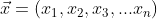
If the point can be described by its coordinates in n dimensions:

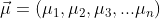
And the distribution has one mean for each independent variable:

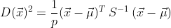
The Mahalanobis Distance (MD) is calculated like this:

The initial term under the square root is the transposed matrix containing the differences between the x’s and the column (independent variable) means. indicates the inverse of the correlation matrix. Fortunately all of these things are easy to calculate in R, and there’s also a function to generate MDs from a multivariate data frame.

This package uses the scaled Mahalanobis Distance recommended by Yang & Trewn (2004):

Steps in MTS Development and Validation

The steps to apply MTS are:

• Create a UNIT SPACE from “good” or “healthy” observations that will form the reference group
  • Select a representative sample of observations and create a data frame containing those observations
  • Normalize the values in the data frame to z-scores
  • Construct a correlation matrix of the normalized values
  • Invert the result
  • Compute one Mahalanobis Distance (MD) for each observation (each row of the data frame)
• Confirm DISCRIMINATORY POWER of MD by doing the same with the “bad” or “unhealthy” observations
  • Calculate MD for the “bad” or “unhealthy” group using procedure above
  • Plot the MDs for the two groups to see if there is discriminatory power (e.g. using a comparative boxplot)
  • You can also plot the sequence of MDs on an I-MR control chart to find where values become “out of bounds”
• Perform FEATURE ENGINEERING to reduce the dataset to the variables that best suggest “good” or “bad” observations
  • This is usually done using a Taguchi orthogonal array based on the number of factors you are considering
  • Recalculate the MDs using subsets of the independent variables (e.g. 8 experimental runs for 4 IVs)
  • For each experimental run, find the average of the SNs for the IVs you used vs. the ones you didn’t use
  • Calculate & plot “gain” for each experimental run (which is the difference between Level 1 and Level 2 means)
  • If the SN drops under the Level 2 condition (that is, not using that particular IV), don’t use that factor
  • Generate the SNs again for your reduced model, and compare how the SNs have changed (e.g. boxplots)
• Collect new observations and USE THE SYSTEM to determine whether new observations are “good” or “bad”
  • Calculate the MD for a new observation and see if it matches the “good” group
  • If not, your observation is “not nominal” – but no way to tell whether it’s super bad or super good

Functions in this Package

• computeMDs - This function computes Mahalanobis Distances (MDs) for “good” and “bad” groups. Takes two arguments: the good data frame, and the bad data frame. They must have one column per predictor/independent variable, and columns must be the same between the two files. The number of rows in each file can, and will usually be, different from one another.
• plotMDs - Plots Mahalanobis Distances from good and bad groups, using index of observation on horizontal axis. Takes as input the output from computeMDs. Optional argument “type” can be hc_scatter or hc_column; default is ggplot bar chart.
• generateTDO - Generates Taguchi Orthogonal Array Design Object (TDO) from an integer number of anticipated predictors/independent variables OR either of the “good” or “bad” data frames of sample observations.
• ltb, stb, dyn.sn - Taguchi Signal-to-Noise formulas for larger-the-better, smaller-the-better, and dynamic (smaller-larger).
• runTaguchi - This function processes the good and bad observations using the TDO as a frame of reference. Yields a data frame with one row per Taguchi experiment, one column per “bad” observation.
• addSN - Adds a Taguchi SN column to output from runTaguchi.
• calcGains - Computes the average SN for each predictor, depending upon whether or not it was used in the Taguchi experiment.
• plotGains - Plots the output of calcGains. Negative gain indicates that the predictor does not enhance the discriminatory power of the MTS. Optional argument “type” can be set to “maineffects” for a maineffects plot across all predictors, “hc_scatter” or “hc_column”. Default is ggplot barplot.
• recommend - Using data frame output from calcGains, this function lists the variables that should be used in the final diagnostic model. Optional argument “type” can be set to “pretty” for aesthetic formatting in Rmd reports.

Example

Here is a quick example using the iris data. This only prepares and plots distances from a collection of good observations and a collection of bad observations. Each collection must have the same number of columns (predictors) but they can have a different number of rows (observations):

library(easyMTS)
library(MASS)
library(dplyr)
library(magrittr)
library(ggplot2)

good <- iris[1:50,1:4]    # Setosa are "healthy" group
bad  <- iris[51:150,1:4]  # Virginica and versicolor are "unhealthy"

mds <- computeMDs(good, bad)
plotMDs(mds)

NicoleRadziwill/easyMTS documentation built on Oct. 30, 2019, 10:14 p.m.