In TiagoOlivoto/WAASB: Multi Environment Trials Analysis
knitr::opts_chunk$set(
  collapse = TRUE,
  comment = "#",
  fig.path = "man/figures/README-"
)
metan 


metan (multi-environment trials analysis) provides useful functions for analyzing multi-environment trial data using parametric and non-parametric methods. The package will help you to:
- Inspect data for possible common errors;
- Manipulate rows and columns;
- Manipulate numbers and strings;
- Manipulate
NAs and 0s;
- Compute descriptive statistics;
- Compute within-environment and joint-analysis of variance;
- Compute AMMI analysis with prediction considering different numbers of interaction principal component axes;
- Compute AMMI-based stability indexes;
- Compute GGE biplot analysis;
- Compute GT and GYT biplot analysis;
- Compute BLUP-based stability indexes;
- Compute variance components and genetic parameters in single environment and multi-environment trials using mixed-effect models;
- Perform cross-validation procedures for AMMI-family and BLUP models;
- Compute parametric and nonparametric stability statistics;
- Implement biometrical models.
Installation
Install the released version of metan from CRAN with:
install.packages("metan")
Or install the development version from GitHub with:
devtools::install_github("TiagoOlivoto/metan")

# To build the HTML vignette use
devtools::install_github("TiagoOlivoto/metan", build_vignettes = TRUE)
Note: If you are a Windows user, you should also first download and install the latest version of Rtools.
For the latest release notes on this development version, see the NEWS file.
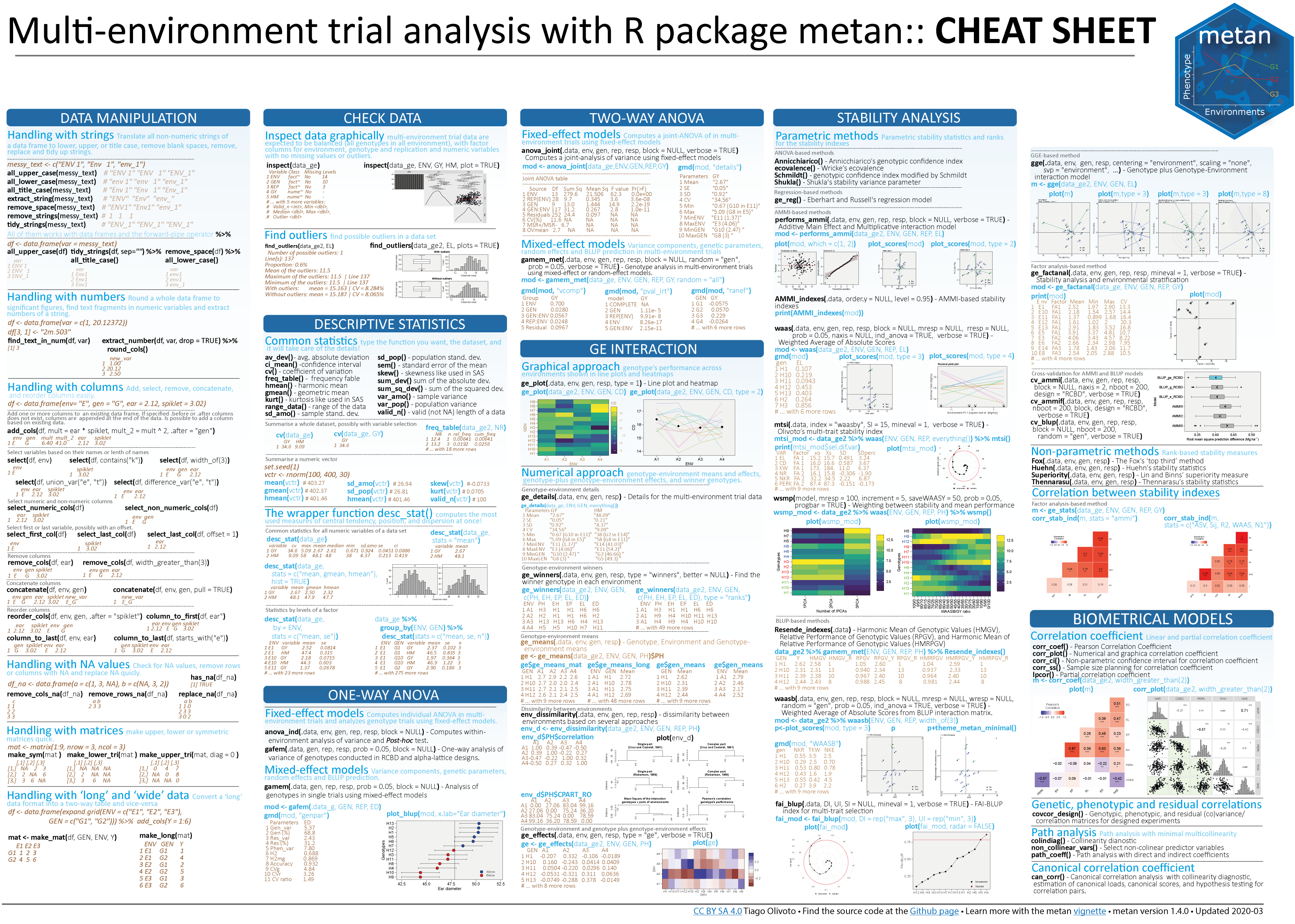
Cheatsheet
Getting started
metan offers a set of functions that can be used to manipulate, summarize, analyze and plot typical multi-environment trial data. Maybe, one of the first functions users should use would be inspect(). Here, we will inspect the example dataset data_ge that contains data on two variables assessed in 10 genotypes growing in 14 environments.
library(metan)
inspect(data_ge, plot = TRUE)
No issues while inspecting the data. If any issue is given here (like outliers, missing values, etc.) consider using find_outliers() to find possible outliers in the data set or any metan's data manipulation tool such as remove_rows_na() to remove rows with NA values, replace_zero() to replace 0's with NA, as_factor() to convert desired columns to factor, find_text_in_num() to find text fragments in columns assumed to be numeric, or even tidy_strings() to tidy up strings.
Descriptive statistics
metan provides a set of functions to compute descriptive statistics. The easiest way to do that is by using desc_stat().
desc_stat(data_ge2)
AMMI model
Fitting the model
The AMMI model is fitted with the function performs_ammi(). To analyze multiple variables at once we can use a comma-separated vector of unquoted variable names, or use any select helper in the argument resp. Here, using everything() we apply the function to all numeric variables in the data. For more details, see the complete vignette.
model <- performs_ammi(data_ge,
                       env = ENV,
                       gen = GEN,
                       rep = REP,
                       resp = everything(),
                       verbose = FALSE)
# Significance of IPCAs
get_model_data(model, "ipca_pval")
Biplots
The well-known AMMI1 and AMMI2 biplots can be created with plot_scores(). Note that since performs_ammi allows analyzing multiple variables at once, e.g., resp = c(v1, v2, ...), the output model is a list, in this case with two elements (GY and HM). By default, the biplots are created for the first variable of the model. To choose another variable use the argument var (e.g., var = "HM").
a <- plot_scores(model)
b <- plot_scores(model,
                 type = 2, # AMMI 2 biplot
                 polygon = TRUE, # show a polygon
                 highlight = c("G4", "G5", "G6"), #highlight genotypes
                 col.alpha.env = 0.5, # alpha for environments
                 col.alpha.gen = 0, # remove the other genotypes
                 col.env = "gray", # color for environment point
                 col.segm.env = "gray", # color for environment segment
                 plot_theme = theme_metan_minimal()) # theme
arrange_ggplot(a, b, tag_levels = "a")
GGE model
The GGE model is fitted with the function gge(). For more details, see the complete vignette.
model <- gge(data_ge, ENV, GEN, GY)
model2 <- gge(data_ge, ENV, GEN, GY, svp = "genotype")
model3 <- gge(data_ge, ENV, GEN, GY, svp = "symmetrical")
a <- plot(model)
b <- plot(model2, type = 8)
c <- plot(model2,
          type = 2,
          col.gen = "black",
          col.env = "gray70",
          axis.expand = 1.5,
          plot_theme = theme_metan_minimal())
arrange_ggplot(a, b, c, tag_levels = "a")
BLUP model
Linear-mixed effect models to predict the response variable in METs are fitted using the function gamem_met(). Here we will obtain the predicted means for genotypes in the variables GY and HM. For more details, see the complete vignette.
model2 <-
  gamem_met(data_ge,
            env = ENV,
            gen = GEN,
            rep = REP,
            resp = everything())
# Get the variance components
get_model_data(model2, what = "vcomp")
Plotting the BLUPs for genotypes
To produce a plot with the predicted means, use the function plot_blup().
a <- plot_blup(model2)
b <- plot_blup(model2,
               prob = 0.2,
               col.shape = c("gray20", "gray80"),
               invert = TRUE)
arrange_ggplot(a, b, tag_levels = "a")
Computing parametric and non-parametric stability indexes
The easiest way to compute parametric and non-parametric stability indexes in metan is by using the function ge_stats(). It is a wrapper function around a lot of specific functions for stability indexes. To get the results into a "ready-to-read" file, use get_model_data() or its shortcut gmd().
stats <- ge_stats(data_ge, ENV, GEN, REP, GY)
get_model_data(stats)
Citation
citation("metan")
Getting help
-
If you encounter a clear bug, please file a minimal reproducible example on github
-
Suggestions and criticisms to improve the quality and usability of the package are welcome!
TiagoOlivoto/WAASB documentation built on March 20, 2024, 4:18 p.m.
R Package Documentation
Browse R Packages
We want your feedback!
Note that we can't provide technical support on individual packages. You should contact the package authors for that.
knitr::opts_chunk$set( collapse = TRUE, comment = "#", fig.path = "man/figures/README-" )
metan
![]()
![]()
metan (multi-environment trials analysis) provides useful functions for analyzing multi-environment trial data using parametric and non-parametric methods. The package will help you to:
- Inspect data for possible common errors;
- Manipulate rows and columns;
- Manipulate numbers and strings;
- Manipulate
NAs and0s; - Compute descriptive statistics;
- Compute within-environment and joint-analysis of variance;
- Compute AMMI analysis with prediction considering different numbers of interaction principal component axes;
- Compute AMMI-based stability indexes;
- Compute GGE biplot analysis;
- Compute GT and GYT biplot analysis;
- Compute BLUP-based stability indexes;
- Compute variance components and genetic parameters in single environment and multi-environment trials using mixed-effect models;
- Perform cross-validation procedures for AMMI-family and BLUP models;
- Compute parametric and nonparametric stability statistics;
- Implement biometrical models.
Installation
Install the released version of metan from CRAN with:
install.packages("metan")
Or install the development version from GitHub with:
devtools::install_github("TiagoOlivoto/metan") # To build the HTML vignette use devtools::install_github("TiagoOlivoto/metan", build_vignettes = TRUE)
Note: If you are a Windows user, you should also first download and install the latest version of Rtools.
For the latest release notes on this development version, see the NEWS file.
Cheatsheet
Getting started
metan offers a set of functions that can be used to manipulate, summarize, analyze and plot typical multi-environment trial data. Maybe, one of the first functions users should use would be inspect(). Here, we will inspect the example dataset data_ge that contains data on two variables assessed in 10 genotypes growing in 14 environments.
library(metan) inspect(data_ge, plot = TRUE)
No issues while inspecting the data. If any issue is given here (like outliers, missing values, etc.) consider using find_outliers() to find possible outliers in the data set or any metan's data manipulation tool such as remove_rows_na() to remove rows with NA values, replace_zero() to replace 0's with NA, as_factor() to convert desired columns to factor, find_text_in_num() to find text fragments in columns assumed to be numeric, or even tidy_strings() to tidy up strings.
Descriptive statistics
metan provides a set of functions to compute descriptive statistics. The easiest way to do that is by using desc_stat().
desc_stat(data_ge2)
AMMI model
Fitting the model
The AMMI model is fitted with the function performs_ammi(). To analyze multiple variables at once we can use a comma-separated vector of unquoted variable names, or use any select helper in the argument resp. Here, using everything() we apply the function to all numeric variables in the data. For more details, see the complete vignette.
model <- performs_ammi(data_ge, env = ENV, gen = GEN, rep = REP, resp = everything(), verbose = FALSE) # Significance of IPCAs get_model_data(model, "ipca_pval")
Biplots
The well-known AMMI1 and AMMI2 biplots can be created with plot_scores(). Note that since performs_ammi allows analyzing multiple variables at once, e.g., resp = c(v1, v2, ...), the output model is a list, in this case with two elements (GY and HM). By default, the biplots are created for the first variable of the model. To choose another variable use the argument var (e.g., var = "HM").
a <- plot_scores(model) b <- plot_scores(model, type = 2, # AMMI 2 biplot polygon = TRUE, # show a polygon highlight = c("G4", "G5", "G6"), #highlight genotypes col.alpha.env = 0.5, # alpha for environments col.alpha.gen = 0, # remove the other genotypes col.env = "gray", # color for environment point col.segm.env = "gray", # color for environment segment plot_theme = theme_metan_minimal()) # theme arrange_ggplot(a, b, tag_levels = "a")
GGE model
The GGE model is fitted with the function gge(). For more details, see the complete vignette.
model <- gge(data_ge, ENV, GEN, GY) model2 <- gge(data_ge, ENV, GEN, GY, svp = "genotype") model3 <- gge(data_ge, ENV, GEN, GY, svp = "symmetrical") a <- plot(model) b <- plot(model2, type = 8) c <- plot(model2, type = 2, col.gen = "black", col.env = "gray70", axis.expand = 1.5, plot_theme = theme_metan_minimal()) arrange_ggplot(a, b, c, tag_levels = "a")
BLUP model
Linear-mixed effect models to predict the response variable in METs are fitted using the function gamem_met(). Here we will obtain the predicted means for genotypes in the variables GY and HM. For more details, see the complete vignette.
model2 <- gamem_met(data_ge, env = ENV, gen = GEN, rep = REP, resp = everything()) # Get the variance components get_model_data(model2, what = "vcomp")
Plotting the BLUPs for genotypes
To produce a plot with the predicted means, use the function plot_blup().
a <- plot_blup(model2) b <- plot_blup(model2, prob = 0.2, col.shape = c("gray20", "gray80"), invert = TRUE) arrange_ggplot(a, b, tag_levels = "a")
Computing parametric and non-parametric stability indexes
The easiest way to compute parametric and non-parametric stability indexes in metan is by using the function ge_stats(). It is a wrapper function around a lot of specific functions for stability indexes. To get the results into a "ready-to-read" file, use get_model_data() or its shortcut gmd().
stats <- ge_stats(data_ge, ENV, GEN, REP, GY) get_model_data(stats)
Citation
citation("metan")
Getting help
-
If you encounter a clear bug, please file a minimal reproducible example on github
-
Suggestions and criticisms to improve the quality and usability of the package are welcome!
R Package Documentation
Browse R Packages
We want your feedback!
Note that we can't provide technical support on individual packages. You should contact the package authors for that.
Embedding an R snippet on your website
Add the following code to your website.
For more information on customizing the embed code, read Embedding Snippets.