inst/examples/appendices/appendices.md

In cboettig/earlywarning: Detection of Early Warning Signals for Catastrophic Bifurcations

This example goes through the steps to demonstrate that in a sufficiently-frequently sampled timeseries, autocorrelation does contain some signal of early warning.

Run the individual based simulation

require(populationdynamics)

Loading required package: populationdynamics

pars = c(Xo = 730, e = 0.5, a = 100, K = 1000, 
    h = 200, i = 0, Da = 0.09, Dt = 0, p = 2)
time = seq(0, 500, length = 500)
sn <- saddle_node_ibm(pars, time)
X <- data.frame(time = time, value = sn$x1)

compute the observed value:

require(earlywarning)

Loading required package: earlywarning

observed <- warningtrend(X, window_autocorr)

fit the models

• ( dX = \alpha(\theta - X) dt + \sigma dB_t )

• ( dX = \gamma_t (\theta - X) dt + \sigma\sqrt(\gamma_t+\theta) dB_t )

A <- stability_model(X, "OU")
B <- stability_model(X, "LSN")

simulate some replicates

reps <- 100
Asim <- simulate(A, reps)
Bsim <- simulate(B, reps)

tidy up the data a bit

require(reshape2)

Loading required package: reshape2

Asim <- melt(Asim, id = "time")
Bsim <- melt(Bsim, id = "time")
names(Asim)[2] <- "rep"
names(Bsim)[2] <- "rep"

Apply the warningtrend window_autocorr to each replicate

require(plyr)

Loading required package: plyr

wsA <- ddply(Asim, "rep", warningtrend, window_autocorr)
wsB <- ddply(Bsim, "rep", warningtrend, window_autocorr)

And gather and plot the results

tidy <- melt(data.frame(null = wsA$tau, test = wsB$tau))

Using  as id variables

names(tidy) <- c("simulation", "value")
require(beanplot)

Loading required package: beanplot

beanplot(value ~ simulation, tidy, what = c(0, 
    1, 0, 0))
abline(h = observed, lty = 2)

require(ggplot2)

Loading required package: ggplot2

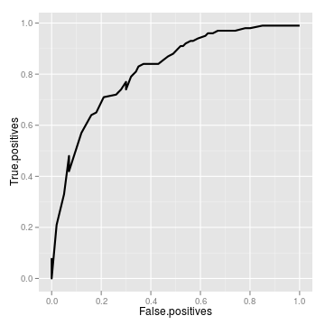
roc <- roc_data(tidy)

Area Under Curve =  0.819680311103255

True positive rate =  0.33 at false positive rate of 0.05

ggplot(roc) + geom_line(aes(False.positives, True.positives), 
    lwd = 1)

Parallelization

Parallel code for the plyr command is straight-forward for multicore use,

require(doMC)

Loading required package: doMC

Loading required package: foreach

Loading required package: iterators

Loading required package: codetools

foreach: simple, scalable parallel programming from Revolution Analytics
Use Revolution R for scalability, fault tolerance and more.
http://www.revolutionanalytics.com

Loading required package: multicore

registerDoMC()
wsA <- ddply(Asim, "rep", warningtrend, window_autocorr, 
    .parallel = TRUE)
wsB <- ddply(Bsim, "rep", warningtrend, window_autocorr, 
    .parallel = TRUE)

Which works nicely (other than the progress indicator finishing early).

In principle, this can be parallelized over MPI using an additional function, seems to work:

library(snow)
library(doSNOW)
source("../createCluster.R")
cl <- createCluster(4, export = ls(), lib = list("earlywarning"))
ws <- ddply(Asim, "rep", warningtrend, window_autocorr, 
    .parallel = TRUE)
stopCluster(cl)
head(ws)

  rep     tau
1  X1  0.7886
2  X2  0.6966
3  X3  0.6543
4  X4  0.5251
5  X5 -0.2859
6  X6 -0.3889

cboettig/earlywarning documentation built on May 13, 2019, 2:07 p.m.