inst/examples/misc_examples/tutorial_with_simulated_traits.md

In cboettig/wrightscape: wrightscape

A wrightscape tutorial using simulated traits

Load package, along with parallelization, plotting, and data manipulation packages. Then load the data.

require(wrightscape)
require(snowfall)
require(ggplot2)
require(reshape)
data(labrids)

rename the regimes less technically

levels(pharyngeal) = c("wrasses", "parrotfish")
regime <- pharyngeal

Create a dataset by simulation, where the parrotfish all have lower alpha

a1_spec <- list(alpha = "indep", sigma = "global", theta = "global")
a1 <- multiTypeOU(data = dat["close"], tree = tree, regimes = regime, 
    model_spec = a1_spec, control = list(maxit = 5000))

## Warning message: mean(<data.frame>) is deprecated.
##  Use colMeans() or sapply(*, mean) instead.

assign expected "startree" standard deviations: wrasses 1.25, parrotfish 5

a1$alpha[1] <- 10
a1$alpha[2] <- 1e-10
a1$sigma <- c(5, 5)
a1$theta <- c(0, 0)
dat[["constraint release"]] <- simulate(a1)[[1]]

Check out the variance in the relative groups -- it should be larger in parrotfish in an extreme example, but need not be in principle, due to the phylogeny.

testcase <- dat[["constraint release"]]
lowvar <- testcase[regime == "wrasses" & !is.na(testcase) & testcase != 
    0]
highvar <- testcase[regime != "wrasses" & !is.na(testcase) & testcase != 
    0]
print(c(var(lowvar), var(highvar)))

## [1] 0.9578 5.5166

We can repeat the whole thing with a model based on differnt sigmas, to make sure

s1_spec <- list(alpha = "global", sigma = "indep", theta = "global")
s1 <- multiTypeOU(data = dat["close"], tree = tree, regimes = pharyngeal, 
    model_spec = s1_spec, control = list(maxit = 5000))

## Warning message: mean(<data.frame>) is deprecated.
##  Use colMeans() or sapply(*, mean) instead.

names(s1$sigma) <- levels(regime)
s1$sigma[1] <- sqrt(2 * 5 * 1.25)
s1$sigma[2] <- sqrt(2 * 5 * 5)
s1$alpha <- c(5, 5)  # We can keep those parameters estimated from data or update them
a1$theta <- c(0, 0)
dat[["faster evolution"]] <- simulate(s1)[[1]]
testcase <- dat[["faster evolution"]]
lowvar <- testcase[regime == "wrasses" & !is.na(testcase) & testcase != 
    0]
highvar <- testcase[regime != "wrasses" & !is.na(testcase) & testcase != 
    0]
print(c(var(lowvar), var(highvar)))

## [1] 1.122 4.417

Now we have a trait where change in alpha is responsible, and one in which sigma change is responsible. Can we correctly identify each??

traits <- c("constraint release", "faster evolution")

fits <- lapply(traits, function(trait) {
    # declare function for shorthand
    multi <- function(modelspec, reps = 20) {
        m <- multiTypeOU(data = dat[[trait]], tree = tree, regimes = pharyngeal, 
            model_spec = modelspec, control = list(maxit = 5000))
        replicate(reps, bootstrap(m))
    }
    bm <- multi(list(alpha = "fixed", sigma = "indep", theta = "global"))
    s1 <- multi(list(alpha = "global", sigma = "indep", theta = "global"))
    a1 <- multi(list(alpha = "indep", sigma = "global", theta = "global"))
    s2 <- multi(list(alpha = "global", sigma = "indep", theta = "indep"))
    a2 <- multi(list(alpha = "indep", sigma = "global", theta = "indep"))
    list(bm = bm, s1 = s1, a1 = a1, s2 = s2, a2 = a2)
})

Reformat and label data for plotting

names(fits) <- traits  # each fit is a different trait (so use it for a label)
data <- melt(fits)
names(data) <- c("regimes", "param", "rep", "value", "model", "trait")

save(list = ls(), file = "tutorial_with_simulated_traits.rda")

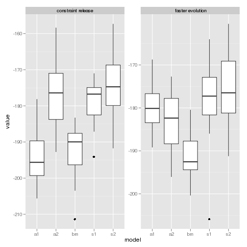
model likelihood

p1 <- ggplot(subset(data, param == "loglik")) + geom_boxplot(aes(model, 
    value)) + facet_wrap(~trait, scales = "free_y")
p1

p2 <- ggplot(subset(data, param %in% c("sigma", "alpha")), aes(model, 
    value, fill = regimes)) + stat_summary(fun.data = mean_sdl, geom = "pointrange", 
    aes(color = regimes), position = position_dodge(width = 0.9)) + scale_y_log10() + 
    facet_grid(param ~ trait, scales = "free_y")
p2

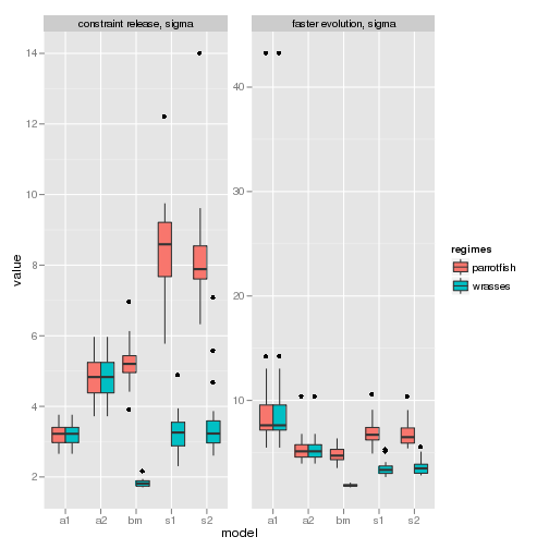
The visualization is easier if we seperate out the plots. Consider focusing on the sigma parameter for both simulations:

p3 <- ggplot(subset(data, param %in% c("sigma"))) + geom_boxplot(aes(model, 
    value, fill = regimes)) + facet_wrap(trait ~ param, scales = "free_y")
p3

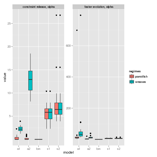
Compare this to the alpha parameter for both simulations:

p4 <- ggplot(subset(data, param %in% c("alpha"))) + geom_boxplot(aes(model, 
    value, fill = regimes)) + facet_wrap(trait ~ param, scales = "free_y")
p4

To really tell these datasets apart, we need the direct model comparison.

save(list = ls(), file = "tutorial_with_simulated_traits.rda")

We'll take advantage of the parallelization inside the montecarlotest function

nboot <- 50
cpu <- 16

require(snowfall)
sfInit(parallel = TRUE, cpu = cpu)

## R Version:  R version 2.15.0 (2012-03-30) 
## 

## snowfall 1.84 initialized (using snow 0.3-8): parallel execution on 16 CPUs.
## 

sfLibrary(wrightscape)

## Library wrightscape loaded.

## Library wrightscape loaded in cluster.
## 

## Warning message: 'keep.source' is deprecated and will be ignored

sfExportAll()

fits <- lapply(traits, function(trait) {
    multi <- function(modelspec) {
        multiTypeOU(data = dat[[trait]], tree = tree, regimes = pharyngeal, 
            model_spec = modelspec, control = list(maxit = 8000))
    }
    bm <- multi(list(alpha = "fixed", sigma = "global", theta = "global"))
    ou <- multi(list(alpha = "global", sigma = "global", theta = "global"))
    bm2 <- multi(list(alpha = "fixed", sigma = "indep", theta = "global"))
    a2 <- multi(list(alpha = "indep", sigma = "global", theta = "global"))
    t2 <- multi(list(alpha = "global", sigma = "global", theta = "indep"))

    mc <- montecarlotest(bm2, a2, cpu = cpu, nboot = nboot)
    bm2_a2 <- list(null = mc$null_dist, test = mc$test_dist, lr = -2 * (mc$null$loglik - 
        mc$test$loglik))
    mc <- montecarlotest(bm, ou, cpu = cpu, nboot = nboot)
    bm_ou <- list(null = mc$null_dist, test = mc$test_dist, lr = -2 * (mc$null$loglik - 
        mc$test$loglik))
    mc <- montecarlotest(bm, bm2, cpu = cpu, nboot = nboot)
    bm_bm2 <- list(null = mc$null_dist, test = mc$test_dist, lr = -2 * (mc$null$loglik - 
        mc$test$loglik))
    mc <- montecarlotest(ou, bm2, cpu = cpu, nboot = nboot)
    ou_bm2 <- list(null = mc$null_dist, test = mc$test_dist, lr = -2 * (mc$null$loglik - 
        mc$test$loglik))
    mc <- montecarlotest(t2, a2, cpu = cpu, nboot = nboot)
    t2_a2 <- list(null = mc$null_dist, test = mc$test_dist, lr = -2 * (mc$null$loglik - 
        mc$test$loglik))
    mc <- montecarlotest(bm2, t2, cpu = cpu, nboot = nboot)
    bm2_t2 <- list(null = mc$null_dist, test = mc$test_dist, lr = -2 * (mc$null$loglik - 
        mc$test$loglik))
    list(brownie_vs_alphas = bm2_a2, brownie_vs_thetas = bm2_t2, thetas_vs_alphas = t2_a2, 
        bm_vs_brownie = bm_bm2, bm_vs_ou = bm_ou, ou_vs_brownie = ou_bm2)
})

Clean up the data

names(fits) <- traits
dat <- melt(fits)
names(dat) <- c("value", "type", "comparison", "trait")

r <- cast(dat, comparison ~ trait, function(x) quantile(x, c(0.1, 
    0.9)))
subdat <- subset(dat, abs(value) < max(abs(as.matrix(r))))

ggplot(subdat) + geom_boxplot(aes(type, value)) + facet_grid(trait ~ 
    comparison, scales = "free_y")

cboettig/wrightscape documentation built on May 13, 2019, 2:12 p.m.