README.md
In eead-csic-eesa/fingerPro: Sediment Source Fingerprinting


FingerPro is a collaborative R project aiming to solve and share all modelling concerns around the sediment fingerprinting technique. Join us and discover the insights of your data!!
The package provides users with tools to i) characterise your database ii) assist in the selection of the optimal tracers moving forward from the traditional tracer selection methods (also included), iii) extract the multiple and consensual solutions in your database and iv) unmix sediment samples to estimate the apportionment of the sediment sources.
The package used state-of-the-art equations and techniques for rigorous unmixing avoiding previous thoughts about only relying on models capacity.
Table of Contents
Table of Contents
- Installation
- Preparing your data
- Visual plots
- Box and whisker plots
- Correlation plot
- 2D and 3D Linear discrimination plot
- Principal component analysis plot
- Novel methods for tracer selection and data understanding
- Conservativeness index (CI) and Ternary plots
- Consensus Ranking approach (CR)
- Consistency based tracer selection
- Video Tutorials :clapper:
- The basics of the technique
- The FingerPro package: A tutorial with code examples
- Citing FingerPro and its tools
- Contributing and feedback
- Related research
For additional details, please see the recently published FingerPro paper and the newly developed tools such as the Consensus Ranking (CR) and the newest developed Consistency based tracer selection (CTS) that includes:
- Full description of functions and how to use them
- Full description of equations
If you're working with stable isotopes or want to combine them with elemental tracers, check the latest published method conservative balance (CB)
:point_right: Frequently Asked Questions :arrow_right: Check them!
Installation
# From CRAN (version 1.1)
install.packages("fingerPro")
library(fingerPro)

# From your computer (version 1.3)
# Download the fingerPro_1.3.zip file from GitHub on your computer. Depending on your version of R, choose one or another.
setwd("C:/your/file/directory")
# install.packages('fingerPro_1.3.zip', repos = NULL) # R 4.1.2
install.packages('fingerPro_1.33.zip', repos = NULL) # R 4.2.1

# From GitHub (version 1.3)
devtools::install_github("eead-csic-eesa/fingerPro", ref = "master", force = T)
Preparing your data
To use your own data is as easy as following the format supplied in the example data included in the fingerPro package
r
 print (catchment)
When using raw data, the following structure needs to be followed
- The first column must be numeric corresponding to the sample ID
- The second column corresponds to the different sources
```r
head (catchment[,c(1:6)])
id Land_Use Pbex K40 Bi214 Ra226
1 42665 AG 9.48 494 31.6 32.9
2 42666 AG 19.12 470 32.2 35.1
3 42667 AG 22.62 513 31.1 28.6
4 42694 AG 24.08 587 32.2 32.9
5 42741 AG 3.38 567 28.2 29.4
6 42770 AG 0.32 586 29.9 31.6
  - Your mixtures must be located in the last rows with the same name in the 2nd column and a different ID (column 1)
 ```r
 tail (catchment[,c(1:6)])
       id   Land_Use  Pbex K40 Bi214 Ra226
17 42705        PI1 51.88 532 25.40 25.90
18 42707        PI1 33.50 530 26.00 24.00
19 42807         SS  0.00 478 26.10 24.30
20 42811         SS  0.00 736 26.20 28.20
21 42812         SS  0.00 607 26.15 26.25
22 42744 mix.sample 24.58 456 26.80 26.90
23 42745 mix.sample 25.58 457 27.80 25.90
 ```

If you only have mean and SD data, follow the format supplied in the Kamish dataset example
```r
sources.file <- system.file("extdata", "Raigani.csv", package = "fingerPro")
data <- read.csv(sources.file)
print(data)
Once you have your data in the appropriate format, load it to your global environment
setwd("C:/Users/.....")
data <- read.table("your dataset.csv", header = T, sep = ',')
Visual plots
The following example displays all the basics commands available in the package to display informative graphs.
If you want to use your own data, see the previous section preparing your data
#Load the dataset called "catchment"
data <- catchment
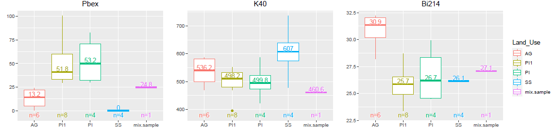
Box and whisker plots
boxPlot(data, columns = 1:3, ncol = 3)
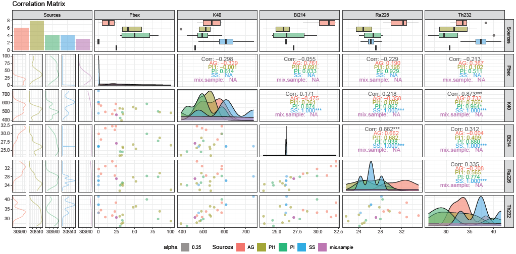
Correlation plot
correlationPlot(data, columns = 1:6, mixtures = T)
2D and 3D Linear discrimination plot
LDAPlot(data[, c(1:10)], P3D = F, text = T)
LDAPlot(data[, c(1:10)], P3D = T)

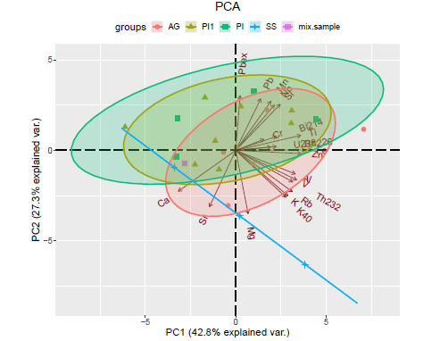
Principal component analysis plot
PCAPlot(data, components = 1:2)
Novel methods for tracer selection and data understanding
Moving forward from the traditionally implemented tracer selection methods proven wrong by recent research, this section explains how to implement state-of-the-art approaches to extract individual tracer information and multiple solutions to assist you in this crucial step.
Major benefits:
- Understanding your dataset
- Are there specific relationships among my tracers?
- Does my dataset has multiple solutions?
- What's leading my model to its results?
- Agreement between different models (e.g. FingerPro & MixSIAR)
Conservativeness index and Ternary plots
sources.file <- system.file("extdata", "Raigani.csv", package = "fingerPro")
data <- read.csv(sources.file)

#Compute the CI index and the individual tracer solutions
results_CI <- CI_Method(data, points = 2000, Means = T) # Means = F (When using raw data)

# Plot the individual tracers solution from the 8 first tracers
Ternary_diagram(results_CI, tracers = c(1:6), n_row = 1, n_col = 6)
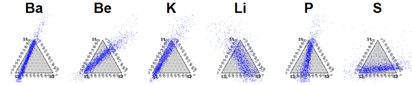
Ternary plots of all possible predictions of each tracer
Consensus Ranking approach

mixture <- tail(data, n = 1)
var <- grep("^D", colnames(data))
mixture <- mixture[-c(var)]
row.names(mixture) <- NULL
source <- head(data,-1)
sgeo <- source[, -1]
mgeo <- mixture[, -1]

# When using raw data
# sgeo <- inputSource(data)
# mgeo <- inputSample(data)

crgeo <- cr_3s(source=sgeo, mixture = mgeo, maxiter = 2000, seed = 1234567)
head(crgeo)

#RESULTS
   tracer score
1       P 96.90
2      Ba 96.45
3      Li 96.00
4       K 95.15
.       .   .
.       .   .
.       .   .
31     Mn  0.85
32     Pb  0.40
33     Cu  0.35
34      V  0.05
Consistency-based tracer selection

# compute pairs/triplets (depending on your source numbers)
pgeo <- pairs(sgeo, mgeo, iter = 2000, seed = 1234567)
head(pgeo)
id w1 w2 w3 Dw1 Dw2 Dw3 cons Dmax
1 Ba Sr 0.6317626 0.09009448 0.278142958 0.05204120 0.03254703 0.04903574 0.9925 0.05204120
2 P Sr 0.5959349 0.20660832 0.197456756 0.05287735 0.04940192 0.04803014 0.9970 0.05287735
3 Sr Th 0.6673848 -0.02575151 0.358366677 0.06000961 0.04818316 0.06068657 0.2840 0.06068657
4 Sr Ti 0.4723578 0.60848947 -0.080847215 0.06102190 0.06848843 0.04681482 0.0455 0.06848843
5 Sr Mg 0.5115884 0.48090866 0.007502897 0.04285354 0.07065800 0.07463573 0.5350 0.07463573
6 K Sr 0.6340332 0.08271014 0.283256639 0.05470178 0.07517778 0.07182738 0.8545 0.07517778
#Explore those pairs (e.g. Ba & Sr)
sol <- pgeo[pgeo$id=="Ba Sr",]
ctsgeo <- cts_3s(source = sgeo, mixture = mgeo, sol = c(sol$w1, sol$w2, sol$w3))
ctsgeo <- ctsgeo %>% right_join(crgeo, by = c("tracer"))
ctsgeo <- ctsgeo[ctsgeo$err < 0.025 & ctsgeo$score > 80,]
print(ctsgeo)
tracer err score
1 Ba 1.110223e-16 96.45
3 K 4.117438e-03 95.15
4 Li 1.541905e-02 96.00
8 Sr 1.998401e-15 93.80
data1 <- select(data,"id","sources","Ba", "Li", "K", "Sr", "DBa", "DLi", "DK", "DSr", "n")
result_FP_1 <- unmix(data1, samples = 200, iter = 200, Means = T)
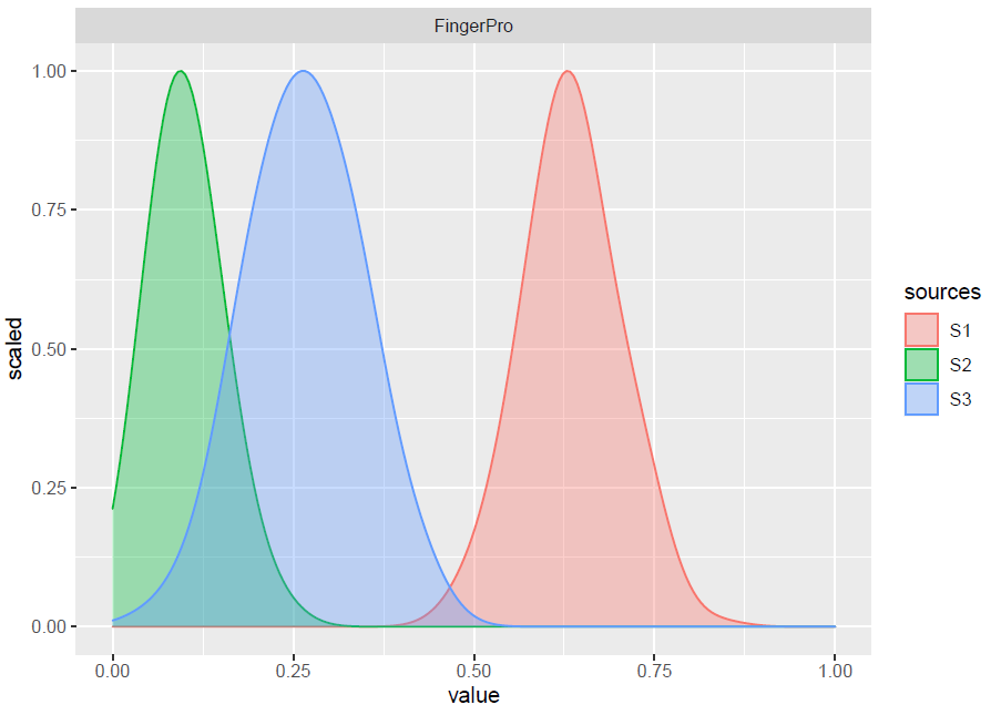
P1 <- plotResults(result_FP_1, y_high = 1)
FingerPro model results from one of the consistent solutions extracted from the CTS method
:clapper: Video Tutorials
The basics of the technique
Also available on bilibili
The FingerPro package

Also available on bilibili
Citing FingerPro and its tools
You can cite this package and the newly developed tools on your work as:
Lizaga, I., Latorre, B., Gaspar, L., Navas, A., 2020. FingerPro: an R package for tracking the provenance of sediment. Water Resources Management 272, 111020. https://doi.org/10.1007/s11269-020-02650-0.
Lizaga, I., Latorre, B., Gaspar, L., Navas, A., 2020a. Consensus ranking as a method to identify non-conservative and dissenting tracers in fingerprinting studies. Science of The Total Environment 720, 137537. https://doi.org/10.1016/j.scitotenv.2020.137537
Latorre, B., Lizaga, I., Gaspar, L., Navas, A., 2021. A novel method for analysing consistency and unravelling multiple solutions in sediment fingerprinting. Science of The Total Environment 789, 147804. https://doi.org/10.1016/j.scitotenv.2021.147804
Lizaga, I., Latorre, B., Gaspar, L., Navas, A., 2022. Combined use of geochemistry and compound-specific stable isotopes for sediment fingerprinting and tracing. Science of The Total Environment 832, 154834. https://doi.org/10.1016/j.scitotenv.2022.154834
and also refer to the code as:
Lizaga I., Latorre B., Gaspar L., Navas A., (2018) fingerPro: An R package for sediment source tracing, https://doi.org/10.5281/zenodo.1402029.
Contributing and feedback
This software has been improved by the questions, suggestions, and bug reports of the user community. If you have any comments, please use the Issues page or report them to lizaga.ivan10@gmail.com.
Related research
- Combining geochemistry and isotopic tracers
- New tools for understanding individual tracers and tracer selection methodologies
- Sediment source fingerprinting in Glacial Landscapes, Svalbard and Peruvian Andes
- Agricultural Cycle influence in sediment and pollutant transport
- Changes in source contribution during an exceptional storm event and before and after the event
- Sediment source fingerprinting in desert environments
- Testing FingerPro model with artificial samples
eead-csic-eesa/fingerPro documentation built on June 28, 2023, 1:39 p.m.
R Package Documentation
Browse R Packages
We want your feedback!
Note that we can't provide technical support on individual packages. You should contact the package authors for that.
![]()
FingerPro is a collaborative R project aiming to solve and share all modelling concerns around the sediment fingerprinting technique. Join us and discover the insights of your data!!
The package provides users with tools to i) characterise your database ii) assist in the selection of the optimal tracers moving forward from the traditional tracer selection methods (also included), iii) extract the multiple and consensual solutions in your database and iv) unmix sediment samples to estimate the apportionment of the sediment sources. The package used state-of-the-art equations and techniques for rigorous unmixing avoiding previous thoughts about only relying on models capacity.
Table of ContentsTable of Contents
- Installation
- Preparing your data
- Visual plots
- Box and whisker plots
- Correlation plot
- 2D and 3D Linear discrimination plot
- Principal component analysis plot
- Novel methods for tracer selection and data understanding
- Conservativeness index (CI) and Ternary plots
- Consensus Ranking approach (CR)
- Consistency based tracer selection
- Video Tutorials :clapper:
- The basics of the technique
- The FingerPro package: A tutorial with code examples
- Citing FingerPro and its tools
- Contributing and feedback
- Related research
For additional details, please see the recently published FingerPro paper and the newly developed tools such as the Consensus Ranking (CR) and the newest developed Consistency based tracer selection (CTS) that includes:
- Full description of functions and how to use them
- Full description of equations
If you're working with stable isotopes or want to combine them with elemental tracers, check the latest published method conservative balance (CB)
:point_right: Frequently Asked Questions :arrow_right: Check them!
Installation
# From CRAN (version 1.1)
install.packages("fingerPro")
library(fingerPro)
# From your computer (version 1.3)
# Download the fingerPro_1.3.zip file from GitHub on your computer. Depending on your version of R, choose one or another.
setwd("C:/your/file/directory")
# install.packages('fingerPro_1.3.zip', repos = NULL) # R 4.1.2
install.packages('fingerPro_1.33.zip', repos = NULL) # R 4.2.1
# From GitHub (version 1.3)
devtools::install_github("eead-csic-eesa/fingerPro", ref = "master", force = T)
Preparing your data
To use your own data is as easy as following the format supplied in the example data included in the fingerPro package
r
print (catchment)
When using raw data, the following structure needs to be followed
- The first column must be numeric corresponding to the sample ID
- The second column corresponds to the different sources
```r
head (catchment[,c(1:6)])
id Land_Use Pbex K40 Bi214 Ra226
1 42665 AG 9.48 494 31.6 32.9
2 42666 AG 19.12 470 32.2 35.1
3 42667 AG 22.62 513 31.1 28.6
4 42694 AG 24.08 587 32.2 32.9
5 42741 AG 3.38 567 28.2 29.4
6 42770 AG 0.32 586 29.9 31.6
- Your mixtures must be located in the last rows with the same name in the 2nd column and a different ID (column 1)
```r
tail (catchment[,c(1:6)])
id Land_Use Pbex K40 Bi214 Ra226
17 42705 PI1 51.88 532 25.40 25.90
18 42707 PI1 33.50 530 26.00 24.00
19 42807 SS 0.00 478 26.10 24.30
20 42811 SS 0.00 736 26.20 28.20
21 42812 SS 0.00 607 26.15 26.25
22 42744 mix.sample 24.58 456 26.80 26.90
23 42745 mix.sample 25.58 457 27.80 25.90
```
If you only have mean and SD data, follow the format supplied in the Kamish dataset example
```r
sources.file <- system.file("extdata", "Raigani.csv", package = "fingerPro")
data <- read.csv(sources.file)
print(data)
Once you have your data in the appropriate format, load it to your global environment
setwd("C:/Users/.....")
data <- read.table("your dataset.csv", header = T, sep = ',')
Visual plots
The following example displays all the basics commands available in the package to display informative graphs.
If you want to use your own data, see the previous section preparing your data
#Load the dataset called "catchment"
data <- catchment
Box and whisker plots
boxPlot(data, columns = 1:3, ncol = 3)
Correlation plot
correlationPlot(data, columns = 1:6, mixtures = T)
2D and 3D Linear discrimination plot
LDAPlot(data[, c(1:10)], P3D = F, text = T)
LDAPlot(data[, c(1:10)], P3D = T)
Principal component analysis plot
PCAPlot(data, components = 1:2)
Novel methods for tracer selection and data understanding
Moving forward from the traditionally implemented tracer selection methods proven wrong by recent research, this section explains how to implement state-of-the-art approaches to extract individual tracer information and multiple solutions to assist you in this crucial step.
Major benefits: - Understanding your dataset - Are there specific relationships among my tracers? - Does my dataset has multiple solutions? - What's leading my model to its results? - Agreement between different models (e.g. FingerPro & MixSIAR)
Conservativeness index and Ternary plots
sources.file <- system.file("extdata", "Raigani.csv", package = "fingerPro")
data <- read.csv(sources.file)
#Compute the CI index and the individual tracer solutions
results_CI <- CI_Method(data, points = 2000, Means = T) # Means = F (When using raw data)
# Plot the individual tracers solution from the 8 first tracers
Ternary_diagram(results_CI, tracers = c(1:6), n_row = 1, n_col = 6)
Ternary plots of all possible predictions of each tracer
Consensus Ranking approach
mixture <- tail(data, n = 1)
var <- grep("^D", colnames(data))
mixture <- mixture[-c(var)]
row.names(mixture) <- NULL
source <- head(data,-1)
sgeo <- source[, -1]
mgeo <- mixture[, -1]
# When using raw data
# sgeo <- inputSource(data)
# mgeo <- inputSample(data)
crgeo <- cr_3s(source=sgeo, mixture = mgeo, maxiter = 2000, seed = 1234567)
head(crgeo)
#RESULTS
tracer score
1 P 96.90
2 Ba 96.45
3 Li 96.00
4 K 95.15
. . .
. . .
. . .
31 Mn 0.85
32 Pb 0.40
33 Cu 0.35
34 V 0.05
Consistency-based tracer selection
# compute pairs/triplets (depending on your source numbers)
pgeo <- pairs(sgeo, mgeo, iter = 2000, seed = 1234567)
head(pgeo)
id w1 w2 w3 Dw1 Dw2 Dw3 cons Dmax
1 Ba Sr 0.6317626 0.09009448 0.278142958 0.05204120 0.03254703 0.04903574 0.9925 0.05204120
2 P Sr 0.5959349 0.20660832 0.197456756 0.05287735 0.04940192 0.04803014 0.9970 0.05287735
3 Sr Th 0.6673848 -0.02575151 0.358366677 0.06000961 0.04818316 0.06068657 0.2840 0.06068657
4 Sr Ti 0.4723578 0.60848947 -0.080847215 0.06102190 0.06848843 0.04681482 0.0455 0.06848843
5 Sr Mg 0.5115884 0.48090866 0.007502897 0.04285354 0.07065800 0.07463573 0.5350 0.07463573
6 K Sr 0.6340332 0.08271014 0.283256639 0.05470178 0.07517778 0.07182738 0.8545 0.07517778
#Explore those pairs (e.g. Ba & Sr)
sol <- pgeo[pgeo$id=="Ba Sr",]
ctsgeo <- cts_3s(source = sgeo, mixture = mgeo, sol = c(sol$w1, sol$w2, sol$w3))
ctsgeo <- ctsgeo %>% right_join(crgeo, by = c("tracer"))
ctsgeo <- ctsgeo[ctsgeo$err < 0.025 & ctsgeo$score > 80,]
print(ctsgeo)
tracer err score
1 Ba 1.110223e-16 96.45
3 K 4.117438e-03 95.15
4 Li 1.541905e-02 96.00
8 Sr 1.998401e-15 93.80
data1 <- select(data,"id","sources","Ba", "Li", "K", "Sr", "DBa", "DLi", "DK", "DSr", "n")
result_FP_1 <- unmix(data1, samples = 200, iter = 200, Means = T)
P1 <- plotResults(result_FP_1, y_high = 1)
FingerPro model results from one of the consistent solutions extracted from the CTS method
:clapper: Video Tutorials
The basics of the technique
Also available on bilibili
The FingerPro package
Also available on bilibili
Citing FingerPro and its tools
You can cite this package and the newly developed tools on your work as:
Lizaga, I., Latorre, B., Gaspar, L., Navas, A., 2020. FingerPro: an R package for tracking the provenance of sediment. Water Resources Management 272, 111020. https://doi.org/10.1007/s11269-020-02650-0.
Lizaga, I., Latorre, B., Gaspar, L., Navas, A., 2020a. Consensus ranking as a method to identify non-conservative and dissenting tracers in fingerprinting studies. Science of The Total Environment 720, 137537. https://doi.org/10.1016/j.scitotenv.2020.137537
Latorre, B., Lizaga, I., Gaspar, L., Navas, A., 2021. A novel method for analysing consistency and unravelling multiple solutions in sediment fingerprinting. Science of The Total Environment 789, 147804. https://doi.org/10.1016/j.scitotenv.2021.147804
Lizaga, I., Latorre, B., Gaspar, L., Navas, A., 2022. Combined use of geochemistry and compound-specific stable isotopes for sediment fingerprinting and tracing. Science of The Total Environment 832, 154834. https://doi.org/10.1016/j.scitotenv.2022.154834
and also refer to the code as:
Lizaga I., Latorre B., Gaspar L., Navas A., (2018) fingerPro: An R package for sediment source tracing, https://doi.org/10.5281/zenodo.1402029.
Contributing and feedback
This software has been improved by the questions, suggestions, and bug reports of the user community. If you have any comments, please use the Issues page or report them to lizaga.ivan10@gmail.com.
Related research
- Combining geochemistry and isotopic tracers
- New tools for understanding individual tracers and tracer selection methodologies
- Sediment source fingerprinting in Glacial Landscapes, Svalbard and Peruvian Andes
- Agricultural Cycle influence in sediment and pollutant transport
- Changes in source contribution during an exceptional storm event and before and after the event
- Sediment source fingerprinting in desert environments
- Testing FingerPro model with artificial samples
R Package Documentation
Browse R Packages
We want your feedback!
Note that we can't provide technical support on individual packages. You should contact the package authors for that.
Embedding an R snippet on your website
Add the following code to your website.
For more information on customizing the embed code, read Embedding Snippets.