README.md

In ezulfica/SANonogramSolver: Nonogram Solver using simulated Annealing

SANonogramSolver

Nonogram Solver using Simulated Annealing

• The generation and transition :
• Random generation :
  • Associated transition :
• Second generation :
  • Associated transition :
• The clues
• The cost function :
• The reason of this metric

Let's talk about nonogram. I like puzzle and I like to think about how to resolve them. This time it's about using Simulated Annealing to solve nonogram.

The thing is, with nonogram. If we set : - n = number of rows * number of columns - k = number of black cells

We can make a lot of combination before solving it, precisely :

number of combination =

This is why we want to Use SA. With the correct optimization, it will be faster to resolve a nonogram than testing all possible combinations. Just a little reminder : since it's using simulated annealing method, it is possible to not obtain the solution by the number of iteration defined.

The generation of the initial state and the associated transition :

It is possible to start with two way :

Random generation :

Firstly we place k black cells randomly.

Associated transition :

We then choose one black cells among the exceeding rows and columns and then change it with an empty cells where it is required to add one cells

nonogram = generate_nonogram(pattern = "boat2")
#pattern = c("random", "penguin", "yinyang" , "boat", "boat2", "fisherman")
r_clues = nonogram$rows_clues
c_clues = nonogram$cols_clues

solve_nonogram(r_clues = r_clues, 
               c_clues = c_clues, 
               n_simul = 50000, 
               beta0 = 0.3, 
               generate = 1, tv = 1, 
               step = 1000, 
               restart = FALSE, 
               plot_result = T, 
               plot_solution = F)

Second generation :

We respect the condition on the rows

Associated transition :

We move the black cells to the right or left only.

nonogram = generate_nonogram(pattern = "penguin")
#pattern = c("random", "penguin", "yinyang" , "boat", "boat2", "fisherman")
r_clues = nonogram$rows_clues
c_clues = nonogram$cols_clues

solve_nonogram(r_clues = r_clues, 
               c_clues = c_clues, 
               n_simul = 50000, 
               beta0 = 0.3, 
               generate = 2, tv = 2, 
               step = 1000, 
               restart = FALSE, 
               plot_result = T, 
               plot_solution = F)

Altought, it is still possible to use the first transition, depending on the situation, it might be slower or stuck in a local minima.

for the plot, i was inspired by coolbutuseless nonogram solver (https://github.com/coolbutuseless/nonogram)

The clues

The clues are in form of list :

example :

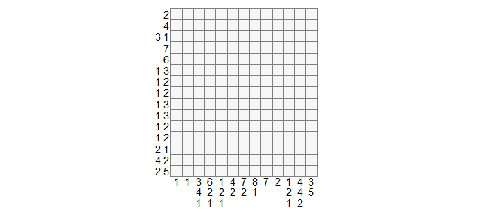
r_clues = list(2, 4, c(3,1), 7, 6, c(1,3), 
               1:2, 1:2,c(1,3), c(1,3), 
               1:2, 1:2, c(2,1), c(4,2), c(2,5)
)
c_clues = list(1, 1, c(3,4,1), c(6,2,1),
               c(1,2,1), c(4,2), c(7,2),
               c(8,1), 7, 2, c(1,2,1), c(4,4,2), c(3,5))

and it's possible to plot an empty grid with the clues :

plot_nonogram(X = 0, r_clues = r_clues, c_clues = c_clues) 
#X = 0 for an empty grid, else put a vector of length n (or an nrows*ncols matrix)

The cost function :

For the cost function, let's suppose we have the solution S :

and a state G :

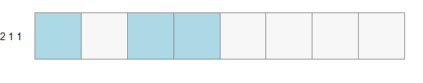
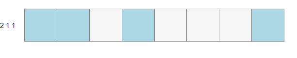
In order to compute the error the maximum number of segments is calculated (NS). For each segments we took the number of black cells, and if the number of segments is lesser than NS, we add zeros.

n_S = (2,1,1)

n_G = (1,2,0)

Then :

Cost = |n_S - n_G| = |2-1| + |1-2| + |1-0| = 3.

We compute every cost by rows and columns (named NB_conflits, which in french mean the number of conflicts)

The reason of this metric

In order to verify whether we have a good cells allocation, our cost function tells us three things : - If we have the required number of cells - If we have the required number of segments - If we have the required number of cells by segments

ezulfica/SANonogramSolver documentation built on Dec. 20, 2021, 7:39 a.m.