README.md

In gersteinlab/siglasso: Optimizing Cancer Mutation Signatures Jointly with Sampling Likelihood

Optimizing Cancer Mutation Signatures Jointly with Sampling Likelihood

Why you should use sigLASSO?

First of all, it is because mutation counts matter. Most other methods, including deconstructSigs, are invariant to different mutation counts. Let's say we observed 10,000 mutations in a cancer sample, this number is large therefore we should have a pretty good estimation of the mutational spectrum of the tumor. Here is a synthetic example.

| Context | Counts | Percentage | | -------- | --- | --- | | AC>AA | 511 | 5.11% | | AC>AC | 305 | 3.05% | | AC>AG | 96 | 0.96% | | AC>AT | 913 | 9.13% | | ... | ... | ... | | TT>GT | 0 | 0 |

But life is not always so good. This time we sequenced another tumor but observed only 100 mutations. It could be because of exome sequencing, shallow sequencing depth or "silent" tumor. Now we are highly unsure about the spectrum.

| Context | Counts | Percentage | | -------- | --- | --- | | AC>AA | 5 | 5% | | AC>AC | 3 | 3% | | AC>AG | 1 | 1% | | AC>AT | 9 | 9% | | ... | ... | ... | | TT>GT | 0 | 0 |

Although the percentage is almost exactly the same as the previous sample, we are much less certain about our spectrum estimation here. For example, in the first sample, with 0/10,000 TT>GT, we are pretty certain that this mutation context is very rare. However, in the second sample, the last zero is very likely due to undersampling rather than a real, very low mutation frequency. Therefore, we should expect these two samples to have two different signature solutions. A more confident one for the first one, and a coarse one for the second sample to reflect the uncertainty in sampling. Most current signature tools will give identical solutions when the percentage matches.

SigLASSO considers both sampling error (especially important when the mutation count is low) and signature fitting.

Moreover, it parameterizes the model empirically. Let the data speak for itself. Moreover, you will be able to feed prior knowledge of the signatures into the model in a soft thresholding way. No more picking up signature subsets by hand! SigLASSO achieves signature selection by using L1 regularization.

Dependencies

To fetch the package from GitHub, you will need "devtools"

install.packages("devtools")
library("devtools")

If start with vcf files, you will additionally need bedtools and a reference genome FASTA file. See the below.

Install

Just one line and voilà!

devtools::install_github("gersteinlab/siglasso")

Usage

It is as simple as 2 (or 3) steps!

0. Starting with VCF

If started with VCF, that is if you do not have the flanking nucleotide context. To make the package transparent and lightweight, we decide to wrap around a bash script to parse mutational context. To do this, you will need bedtools(https://bedtools.readthedocs.io). For Mac OS, I find package managers, like homebrew(https://brew.sh/), greatly simplify the installation.

brew install bedtools

Then you also need to have an uncompressed reference genome that is compatible with your vcf ready.

Before running, one last thing is to prepare a meta file specify the paths of all your vcf files. An optional 2nd column can be used to specify sample names. Otherwise, it will grab the filenames as sample names.

/Users/data/breast/brca_cancer_1.vcf, brca_a_1
/Users/data/breast/brca_cancer_1.vcf, brca_b_1
/Users/data/prostate/prca_cancer_1.vcf, prca_c_1

Run

my_spectrum <- vcf2spec(bedtools_path, vcf_meta, ref_genome, output_file, ...)

This function will write "output_file" to disk. It is a context file.

1. Starting with a context file

Alternatively, you can start with a context file. It is easier when you already know the flanking region context. Many annotation tools now give you this.

The context file has three columns. The 1st column is the reference nucleotide context. Typically, it is a trinucleotide. The 2nd column stores the alternative alleles. The last column has the sample names (can be unordered).

ATT    C    brca_a_1
CGT    C    brca_a_2
TCC    A    brca_a_1

Now convert this raw mutation context file into a spectrum.

my_context_file <- read.table(path_to_context_file)
my_spectrum <- context2spec(my_context_file)

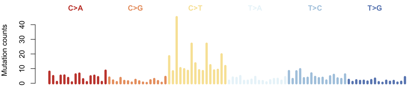
The package comes with an example of 7 AML mutations downloaded from ftp://ftp.sanger.ac.uk/pub/cancer/AlexandrovEtAl (Alexandrovet al., 2013). It contains 3,414 SNVs, already in the context file format.

data(aml_7_wgs)
my_spectrum <- context2spec(aml_7_wgs)

It will make plots of the spectrum, to know more, see plot_spectrum()

Note: the specturm could be further "normalized". But the COSMIC signatures are built on a mixture of WGS and WES samples, it is unclear such normarlization will provide any advantage. Meanwhile, normalization here destroyed the discrete nature of the mutation counts. So please do not use normarlized spectrum as input for siglasso (step 2). siglasso() provides a normalization option applied to the signatures (which is not recommended either for COSMIC signatures).

2. Apply siglasso to spectrum

This step is straightforward. You can supply your own signature file, or it will use the COSMIC signature.

my_sigs <- siglasso(my_spectrum, ...)

A useful thing is prior. Pass a vector of the length of the number of signatures, with numbers between 0 (strong preference, we recommend using a small number, e.g. 0.01, rather than 0) and 1 (no preference). We supply a prior file that we curated from COSMIC. The prior file consists of binary indicators of a signature is observed in COSMIC studies (value: 0) or not (value: 1). To apply an easy flat prior on previously observed signatures, just multiple the prior vector with a value less than 1. Here is an example.

data(cosmic_priors)
colnames(cosmic_priors)
my_prior = ifelse(cosmic_priors$BRCA==0, 0.1, 1) #adjust the strength to 0.1, BRCA
my_sigs <- siglasso(my_spectrum, prior = my_prior[1:30]...) #the last row is "other signatures"

3. Visualization

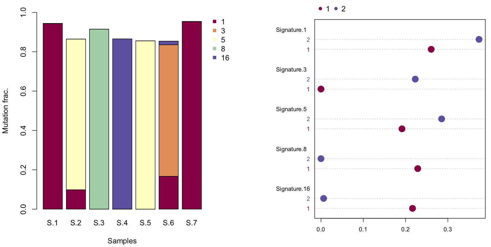
By default, siglasso() automatically generates a barplot of every sample

plot_sigs(my_sigs, ...)

There is another option to generate a dotchart to compare between samples or samples groups. For illustration, we randomly group the first four samples and the last three into group 1 & 2.

plot_sigs_grouped(my_sigs, c(rep(1,4), rep(2,3))...)

4. Documentation

You can use the build-in documentation in R, or download a pdf version of the pacakge manual at (http://labmisc.gersteinlab.org/siglasso_1.1.pdf)

Longer Introduction

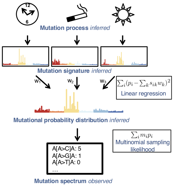
Multiple mutational processes drive carcinogenesis, leaving characteristic signatures on tumor genomes. Determining the active signatures from the full repertoire of potential ones can help elucidate mechanisms underlying cancer initiation and development. This task involves decomposing the counts of cancer mutations, tabulated according to their trinucleotide context, into a linear combination of known mutational signatures. We formulate it as an optimization problem and develop sigLASSO, a software tool, to carry it out efficiently. SigLASSO features four key aspects: (1) It jointly optimizes the likelihood of sampling and signature fitting, by explicitly adding multinomial sampling into the overall objective function, This is particularly important when mutation counts are low and sampling variance is high, such as in exome sequencing. (2) sigLASSO uses L1 regularization to parsimoniously assign signatures to mutation profiles, leading to sparse and more biologically interpretable solutions resembling previously well-characterized results. (3) sigLASSO fine-tunes model complexity, informed by the scale of the data and biological-knowledge based priors. In particular, instead of hard thresholding and choosing a priori a discrete subset of active signatures, sigLASSO allows continuous priors, which can be effectively learned from auxiliary information. (4) Because of this, sigLASSO can assess model uncertainty and abstain from making certain assignments in low-confidence contexts. Finally, to evaluate SigLASSO signature assignments in comparison to other approaches, we develop a set of reasonable expectations (e.g. sparsity, the ability to abstain, and robustness to noise) that we apply consistently in a variety of contexts.

Citation

This work is accepted by Nature Communications, please cite https://doi.org/10.1038/s41467-020-17388-x

Data

Download sigLASSO output on TCGA samples with COSMIC (v2) priors (http://labmisc.gersteinlab.org/all_sigs.tsv.tar.gz)

What is new

version 1.1 (2020 April) Support for the newest COSMIC signature v3 (both whole genome and exome) Also better visualization support

gersteinlab/siglasso documentation built on Sept. 5, 2022, 8:45 p.m.