In lgnbhl/BFS: Get Data from the Swiss Federal Statistical Office


BFS 
knitr::opts_chunk$set(
    echo = TRUE,
    message = FALSE,
    warning = FALSE
)
Search and download data from the Swiss Federal Statistical Office
The BFS package allows to search and download public data from the
Swiss Federal Statistical Office{target="_blank"} (BFS stands for Bundesamt für Statistik in German) APIs in a dynamic and reproducible way.
Installation
install.packages("BFS")
You can also install the development version from Github.
devtools::install_github("lgnbhl/BFS")
Usage
library(BFS)
Get the data catalog
Retrieve the list of publicly available datasets from the data catalog in any language ("de", "fr", "it" or "en") by calling bfs_get_catalog_data().
bfs_get_catalog_data(language = "en")
You can search in the data catalog using the following arguments:
language: The language of a BFS catalog, i.e. "de", "fr", "it" or "en".title: to search in title, subtitle and supertitle.extended_search: extended search in (sub/super)title, orderNr, summary, shortSummary, shortTextGNP.spatial_division: choose between "Switzerland", "Cantons", "Districts", "Communes", "Other spatial divisions" or "International".prodima: by specific BFS themes using a unique prodima number.inquiry: by inquiry number.institution: by institution.publishing_year_start: by publishing year start.publishing_year_end: by publishing year end.order_nr: by BFS Number (FSO number).
For example, you can search data related to students using the extend search:
catalog_student <- bfs_get_catalog_data(language = "en", extended_search = "student")

catalog_student
Note the the BFS number (FSO number) is available in column order_nr.
English ("en") and Italian ("it") data catalogs offer a limited list of datasets. For the full list please get the French ("fr") or German ("de") data catalogs (see language_available column).
Download data in any language
The function bfs_get_data() allows you to download any dataset from the data catalog using its BFS number (FSO number).
Using the number_bfs argument (FSO number), you can get BFS data in a given language ("en", "de", "fr" or "it") from the official PXWeb API of the Swiss Federal Statistical Office.
#catalog_student$order_nr[1] # px-x-1502040100_131

bfs_get_data(number_bfs = "px-x-1502040100_131", language = "en")
"Too Many Requests" error message
When running the bfs_get_data() function you may get the following error message (issue #7).
Error in pxweb_advanced_get(url = url, query = query, verbose = verbose) :
  Too Many Requests (RFC 6585) (HTTP 429).
This could happen because you ran too many times a bfs_get_*() function (API config is here). A solution is to wait a few seconds before running the next bfs_get_*() function. You can add a delay in your R code using the delay argument.
bfs_get_data(
  number_bfs = "px-x-1502040100_131",
  language = "en",
  delay = 10
)
If the error message remains, it could be because you are querying a very large BFS dataset. Two workarounds exist: a) download the BFS file using bfs_download_asset() to read it locally or b) query only specific elements of the data to reduce the API call (see next section).
Here an example using the bfs_download_asset() function:
BFS::bfs_download_asset(
  number_bfs = "px-x-1502040100_131", #number_asset also possible
  destfile = "px-x-1502040100_131.px"
)

library(pxR) # install.packages("pxR")
large_dataset <- pxR::read.px(filename = "px-x-1502040100_131.px") |>
  as.data.frame()
Note that reading a PX file using pxR::read.px() gives access only to the German version.
Query specific elements
First you want to get the metadata of your dataset, i.e. the variables (code and text) and dimensions (values and valueTexts). For example:
metadata <- bfs_get_metadata(number_bfs = "px-x-1502040100_131", language = "en")

# tidy metadata
library(dplyr)
library(tidyr) # for unnest_longer

metadata_tidy <- metadata |>
  unnest_longer(c(values, valueTexts))

metadata_tidy
## # A tibble: 92 × 7
##    code  text  values valueTexts time  elimination
##    <chr> <chr> <chr>  <chr>      <lgl> <lgl>
##  1 Jahr  Year  0      1980/81    TRUE  NA
##  2 Jahr  Year  1      1981/82    TRUE  NA
##  3 Jahr  Year  2      1982/83    TRUE  NA
##  4 Jahr  Year  3      1983/84    TRUE  NA
##  5 Jahr  Year  4      1984/85    TRUE  NA
##  6 Jahr  Year  5      1985/86    TRUE  NA
##  7 Jahr  Year  6      1986/87    TRUE  NA
##  8 Jahr  Year  7      1987/88    TRUE  NA
##  9 Jahr  Year  8      1988/89    TRUE  NA
## 10 Jahr  Year  9      1989/90    TRUE  NA
## # ℹ 82 more rows
## # ℹ 1 more variable: title <chr>
Then you can filter the dimensions you want to query using the text and valueTexts variables and build the query dimension object with the code and values variables.
# select dimensions
dim1 <- metadata_tidy |>
  filter(text == "Year" & valueTexts %in% c("2020/21", "2021/22"))
dim2 <- metadata_tidy |>
  filter(text == "Level of study" & valueTexts %in% c("Master", "Doctorate"))
dim3 <- metadata_tidy |>
  filter(text == "ISCED Field" & valueTexts %in% c("Education science"))
dim4 <- metadata_tidy |>
  filter(text == "Sex") # all valueTexts dimensions

# build dimensions list object
dimensions <- list(
  dim1$values,
  dim2$values,
  dim3$values,
  dim4$values
)

names(dimensions) <- c(
  unique(dim1$code),
  unique(dim2$code),
  unique(dim3$code),
  unique(dim4$code)
)

dimensions
## $Jahr
## [1] "40" "41"
##
## $Studienstufe
## [1] "2" "3"
##
## $`ISCED Fach`
## [1] "0"
##
## $Geschlecht
## [1] "0" "1"
Finally you can query BFS data with specific dimensions.
BFS::bfs_get_data(
  number_bfs = "px-x-1502040100_131",
  language = "en",
  query = dimensions
  )
## # A tibble: 8 × 5
##   Year    `ISCED Field`     Sex    `Level of study` `University students`
##   <chr>   <chr>             <chr>  <chr>                            <dbl>
## 1 2020/21 Education science Male   Master                             151
## 2 2020/21 Education science Male   Doctorate                          121
## 3 2020/21 Education science Female Master                             555
## 4 2020/21 Education science Female Doctorate                          306
## 5 2021/22 Education science Male   Master                             143
## 6 2021/22 Education science Male   Doctorate                          115
## 7 2021/22 Education science Female Master                             599
## 8 2021/22 Education science Female Doctorate                          318
Catalog of tables
A lot of datasets are not accessible through the official PXWeb API. They are listed in the catalog of tables. You can search for specific tables using bfs_get_catalog_tables().
catalog_tables_en_students <- bfs_get_catalog_tables(language = "en", title = "students")

catalog_tables_en_students
## # A tibble: 5 × 7
##   title              language publication_date    number_asset url_bfs url_table
##   <chr>              <chr>    <dttm>                     <dbl> <chr>   <chr>
## 1 Students at unive… en       2023-04-05 00:00:00     24865589 https:… https://…
## 2 Students at unive… en       2023-04-05 00:00:00     24865590 https:… https://…
## 3 Students at unive… en       2023-03-28 08:30:00     24345362 https:… https://…
## 4 Students at unive… en       2023-03-28 08:30:00     24345374 https:… https://…
## 5 Students at unive… en       2023-03-28 08:30:00     24345366 https:… https://…
## # ℹ 1 more variable: catalog_date <dttm>
Most of the BFS tables are Excel or CSV files. You can download an table with bfs_download_asset() using the number asset.
library(dplyr)

tables_asset_number_students <- catalog_tables_en_students |>
  dplyr::filter(title == "Students at universities and institutes of technology: Basistables") |>
  dplyr::pull(number_asset)

file_path <- BFS::bfs_download_asset(
  number_asset = tables_asset_number_students,
  destfile = "su-e-15.02.04.01.xlsx"
)
Access geodata catalog
Display geo-information catalog of the Swiss Official STAC API using bfs_get_catalog_geodata().
catalog_geodata <- bfs_get_catalog_geodata(include_metadata = TRUE)

catalog_geodata
## # A tibble: 281 × 12
##    collection_id     type  href  title description created updated crs   license
##    <chr>             <chr> <chr> <chr> <chr>       <chr>   <chr>   <chr> <chr>
##  1 ch.are.agglomera… API   http… Citi… "The list … 2021-1… 2023-0… http… propri…
##  2 ch.are.alpenkonv… API   http… Alpi… "The perim… 2021-1… 2022-0… http… propri…
##  3 ch.are.belastung… API   http… Load… "Passenger… 2021-1… 2022-0… http… propri…
##  4 ch.are.belastung… API   http… Load… "Passenger… 2021-1… 2022-0… http… propri…
##  5 ch.are.belastung… API   http… Load… "Vehicles … 2021-1… 2022-0… http… propri…
##  6 ch.are.belastung… API   http… Load… "Vehicles … 2021-1… 2022-0… http… propri…
##  7 ch.are.erreichba… API   http… Acce… "Accessibi… 2021-1… 2022-0… http… propri…
##  8 ch.are.erreichba… API   http… Acce… "Accessibi… 2021-1… 2022-0… http… propri…
##  9 ch.are.gemeindet… API   http… Typo… "The typol… 2021-1… 2022-0… http… propri…
## 10 ch.are.gueteklas… API   http… Publ… "The publi… 2021-1… 2023-0… http… propri…
## # ℹ 271 more rows
## # ℹ 3 more variables: provider_name <chr>, bbox <list>, inverval <list>
Download geodata
For example you can get information about the dataset "Generalised borders G1 and area with urban character".
library(dplyr)

geodata_g1 <- catalog_geodata |>
  filter(title == "Generalised borders G1 and area with urban character")

geodata_g1
## # A tibble: 1 × 12
##   collection_id      type  href  title description created updated crs   license
##   <chr>              <chr> <chr> <chr> <chr>       <chr>   <chr>   <chr> <chr>
## 1 ch.bfs.generalisi… API   http… Gene… Administra… 2022-0… 2023-0… http… propri…
## # ℹ 3 more variables: provider_name <chr>, bbox <list>, inverval <list>
Download dataset by collection id with bfs_download_geodata() and unzip file if needed.
# Access Generalised borders G1 and area with urban character
borders_g1_path <- bfs_download_geodata(
  collection_id = "ch.bfs.generalisierte-grenzen_agglomerationen_g1",
  output_dir = tempdir() #  temporary directory
)

# you may need to unzip the file
unzip(borders_g1_path[4], exdir = "borders_G1")
By default, the files are downloaded in a temporary directory. You can specify the folder where saving the files using the output_dir argument.
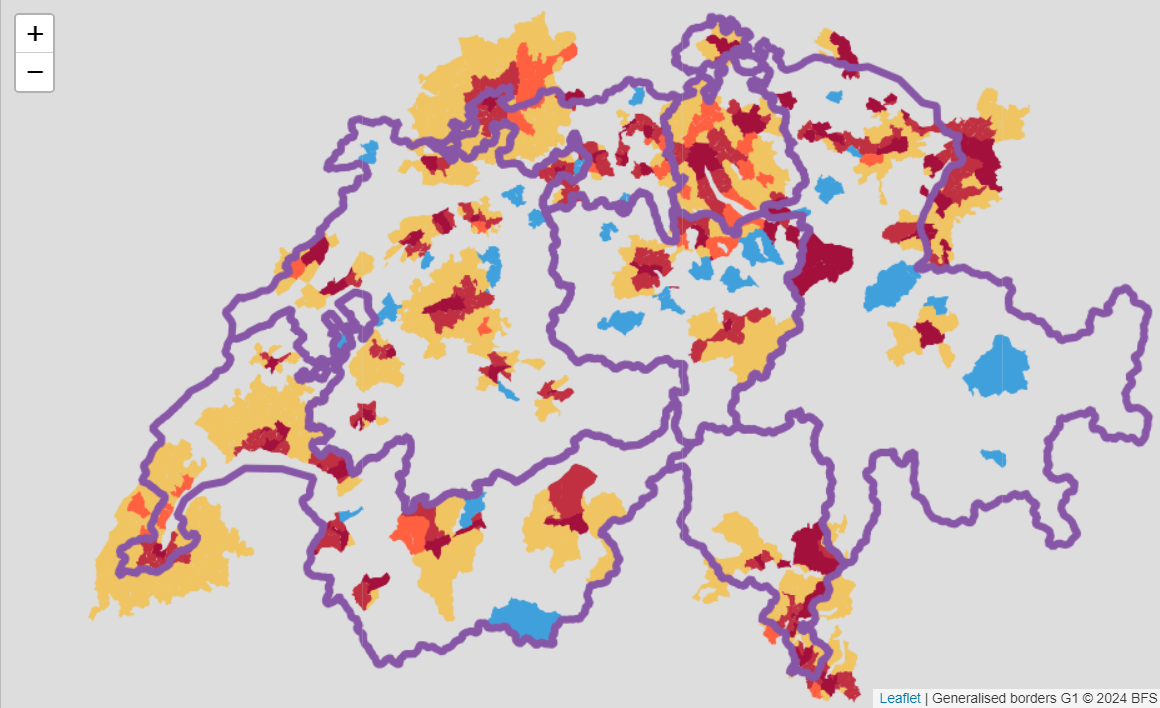
Some layers are accessible using WMS (Web Map Service):
library(leaflet)

leaflet() %>%
  setView(lng = 8, lat = 46.8, zoom = 8) %>%
  addWMSTiles(
    baseUrl = "https://wms.geo.admin.ch/?",
    layers = "ch.bfs.generalisierte-grenzen_agglomerationen_g2",
    options = WMSTileOptions(format = "image/png", transparent = TRUE),
    attribution = "Generalised borders G1 © 2024 BFS")
Cartographic base maps
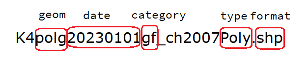
You can get cartographic base maps from the ThemaKart project using bfs_get_base_maps(). The list of available geometries in the official documentation.
The default arguments of bfs_get_base_maps() can be change to access specific files:
# default arguments
bfs_get_base_maps(
  geom = NULL,
  category = "gf", # "gf" for total area (i.e. "Gesamtflaeche")
  type = "Poly",
  date = NULL,
  most_recent = TRUE, #get most recent file by default
  format = "shp",
  asset_number = "24025646" #change to get older ThemaKart data
)
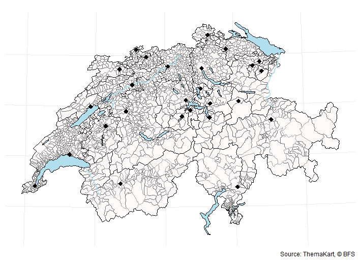
A typical base maps ThemaKart file looks like this:
# list of geometry names: https://www.bfs.admin.ch/asset/en/24025645
switzerland_sf <- bfs_get_base_maps(geom = "suis")
communes_sf <- bfs_get_base_maps(geom = "polg", date = "20230101")
districts_sf <- bfs_get_base_maps(geom = "bezk")
cantons_sf <- bfs_get_base_maps(geom = "kant")
cantons_capitals_sf <- bfs_get_base_maps(geom = "stkt", type = "Pnts", category = "kk")
lakes_sf <- bfs_get_base_maps(geom = "seen", category = "11")

library(ggplot2)

ggplot() +
  geom_sf(data = communes_sf, fill = "snow", color = "grey45") +
  geom_sf(data = lakes_sf, fill = "lightblue2", color = "black") +
  geom_sf(data = districts_sf, fill = "transparent", color = "grey65") +
  geom_sf(data = cantons_sf, fill = "transparent", color = "black") +
  geom_sf(data = cantons_capitals_sf, shape = 18, size = 3) +
  theme_minimal() +
  theme(axis.text = element_blank()) +
  labs(caption = "Source: ThemaKart, © BFS")
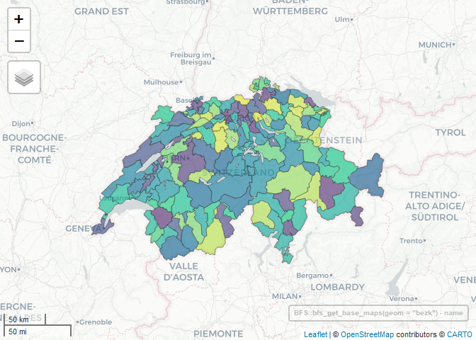
You can create an interactive map easily with the mapview R package.
library(mapview)

BFS::bfs_get_base_maps(geom = "bezk") |>
  mapview(zcol = "name", legend = FALSE)
Swiss Official Commune Register
The package also contains the official Swiss official commune registers for different administrative levels:
register_gderegister_gde_otherregister_bznregister_ktregister_kt_seeanteileregister_dic
# commune register data
BFS::register_gde
You can use registers to ease geodata analysis.
library(dplyr)
library(sf)

communes_sf <- bfs_get_base_maps(geom = "polg", date = "20230101")

communes_ge <- communes_sf |>
  inner_join(BFS::register_gde |>
               filter(GDEKTNA == "Genève"),
             by = c("id" = "GDENR"))

bbox_ge <- sf::st_bbox(communes_ge)

lake_leman <- bfs_get_base_maps(geom = "seen", category = "11") |>
  filter(name == "Lac Léman")

communes_ge |>
  ggplot() +
  geom_sf(data = lake_leman, fill = "lightblue2", color = "grey65") +
  geom_sf(fill = "snow", color = "grey65") +
  geom_sf_text(aes(label = name), size = 3, check_overlap = T) +
  # bounding box
  coord_sf(
    xlim = c(bbox_ge$xmin, bbox_ge$xmax),
    ylim = c(bbox_ge$ymin, bbox_ge$ymax)
  ) +
  theme_minimal() +
  theme(axis.text = element_blank()) +
  labs(title = "Communes du canton de Genève",
       x = NULL, y = NULL,
       caption = "Source: ThemaKart, © BFS")
Main dependencies of the package
Under the hood, this package is using the pxweb{target="_blank"} package to query the Swiss Federal Statistical Office PXWEB API. PXWEB is an API structure developed by Statistics Sweden and other national statistical institutions (NSI) to disseminate public statistics in a structured way. To query the Geo Admin STAC API, this package is using the rstac package. STAC is a specification of files and web services used to describe geospatial information assets.
You can clean the column names of the datasets automatically using janitor::clean_names() by adding the argument clean_names = TRUE in the bfs_get_data() function.
Other information
This package is in no way officially related to or endorsed by the Swiss Federal Statistical Office (BFS).
Contribute
Any contribution is strongly appreciated. Feel free to report a bug, ask any question or make a pull request for any remaining issue.
lgnbhl/BFS documentation built on Sept. 26, 2024, 4:18 p.m.
R Package Documentation
Browse R Packages
We want your feedback!
Note that we can't provide technical support on individual packages. You should contact the package authors for that.
![]()
![]()
BFS
knitr::opts_chunk$set( echo = TRUE, message = FALSE, warning = FALSE )
Search and download data from the Swiss Federal Statistical Office
The BFS package allows to search and download public data from the
Swiss Federal Statistical Office{target="_blank"} (BFS stands for Bundesamt für Statistik in German) APIs in a dynamic and reproducible way.
Installation
install.packages("BFS")
You can also install the development version from Github.
devtools::install_github("lgnbhl/BFS")
Usage
library(BFS)
Get the data catalog
Retrieve the list of publicly available datasets from the data catalog in any language ("de", "fr", "it" or "en") by calling bfs_get_catalog_data().
bfs_get_catalog_data(language = "en")
You can search in the data catalog using the following arguments:
language: The language of a BFS catalog, i.e. "de", "fr", "it" or "en".title: to search in title, subtitle and supertitle.extended_search: extended search in (sub/super)title, orderNr, summary, shortSummary, shortTextGNP.spatial_division: choose between "Switzerland", "Cantons", "Districts", "Communes", "Other spatial divisions" or "International".prodima: by specific BFS themes using a unique prodima number.inquiry: by inquiry number.institution: by institution.publishing_year_start: by publishing year start.publishing_year_end: by publishing year end.order_nr: by BFS Number (FSO number).
For example, you can search data related to students using the extend search:
catalog_student <- bfs_get_catalog_data(language = "en", extended_search = "student") catalog_student
Note the the BFS number (FSO number) is available in column order_nr.
English ("en") and Italian ("it") data catalogs offer a limited list of datasets. For the full list please get the French ("fr") or German ("de") data catalogs (see language_available column).
Download data in any language
The function bfs_get_data() allows you to download any dataset from the data catalog using its BFS number (FSO number).
Using the number_bfs argument (FSO number), you can get BFS data in a given language ("en", "de", "fr" or "it") from the official PXWeb API of the Swiss Federal Statistical Office.
#catalog_student$order_nr[1] # px-x-1502040100_131 bfs_get_data(number_bfs = "px-x-1502040100_131", language = "en")
"Too Many Requests" error message
When running the bfs_get_data() function you may get the following error message (issue #7).
Error in pxweb_advanced_get(url = url, query = query, verbose = verbose) : Too Many Requests (RFC 6585) (HTTP 429).
This could happen because you ran too many times a bfs_get_*() function (API config is here). A solution is to wait a few seconds before running the next bfs_get_*() function. You can add a delay in your R code using the delay argument.
bfs_get_data( number_bfs = "px-x-1502040100_131", language = "en", delay = 10 )
If the error message remains, it could be because you are querying a very large BFS dataset. Two workarounds exist: a) download the BFS file using bfs_download_asset() to read it locally or b) query only specific elements of the data to reduce the API call (see next section).
Here an example using the bfs_download_asset() function:
BFS::bfs_download_asset( number_bfs = "px-x-1502040100_131", #number_asset also possible destfile = "px-x-1502040100_131.px" ) library(pxR) # install.packages("pxR") large_dataset <- pxR::read.px(filename = "px-x-1502040100_131.px") |> as.data.frame()
Note that reading a PX file using pxR::read.px() gives access only to the German version.
Query specific elements
First you want to get the metadata of your dataset, i.e. the variables (code and text) and dimensions (values and valueTexts). For example:
metadata <- bfs_get_metadata(number_bfs = "px-x-1502040100_131", language = "en") # tidy metadata library(dplyr) library(tidyr) # for unnest_longer metadata_tidy <- metadata |> unnest_longer(c(values, valueTexts)) metadata_tidy
## # A tibble: 92 × 7 ## code text values valueTexts time elimination ## <chr> <chr> <chr> <chr> <lgl> <lgl> ## 1 Jahr Year 0 1980/81 TRUE NA ## 2 Jahr Year 1 1981/82 TRUE NA ## 3 Jahr Year 2 1982/83 TRUE NA ## 4 Jahr Year 3 1983/84 TRUE NA ## 5 Jahr Year 4 1984/85 TRUE NA ## 6 Jahr Year 5 1985/86 TRUE NA ## 7 Jahr Year 6 1986/87 TRUE NA ## 8 Jahr Year 7 1987/88 TRUE NA ## 9 Jahr Year 8 1988/89 TRUE NA ## 10 Jahr Year 9 1989/90 TRUE NA ## # ℹ 82 more rows ## # ℹ 1 more variable: title <chr>
Then you can filter the dimensions you want to query using the text and valueTexts variables and build the query dimension object with the code and values variables.
# select dimensions dim1 <- metadata_tidy |> filter(text == "Year" & valueTexts %in% c("2020/21", "2021/22")) dim2 <- metadata_tidy |> filter(text == "Level of study" & valueTexts %in% c("Master", "Doctorate")) dim3 <- metadata_tidy |> filter(text == "ISCED Field" & valueTexts %in% c("Education science")) dim4 <- metadata_tidy |> filter(text == "Sex") # all valueTexts dimensions # build dimensions list object dimensions <- list( dim1$values, dim2$values, dim3$values, dim4$values ) names(dimensions) <- c( unique(dim1$code), unique(dim2$code), unique(dim3$code), unique(dim4$code) ) dimensions
## $Jahr ## [1] "40" "41" ## ## $Studienstufe ## [1] "2" "3" ## ## $`ISCED Fach` ## [1] "0" ## ## $Geschlecht ## [1] "0" "1"
Finally you can query BFS data with specific dimensions.
BFS::bfs_get_data( number_bfs = "px-x-1502040100_131", language = "en", query = dimensions )
## # A tibble: 8 × 5 ## Year `ISCED Field` Sex `Level of study` `University students` ## <chr> <chr> <chr> <chr> <dbl> ## 1 2020/21 Education science Male Master 151 ## 2 2020/21 Education science Male Doctorate 121 ## 3 2020/21 Education science Female Master 555 ## 4 2020/21 Education science Female Doctorate 306 ## 5 2021/22 Education science Male Master 143 ## 6 2021/22 Education science Male Doctorate 115 ## 7 2021/22 Education science Female Master 599 ## 8 2021/22 Education science Female Doctorate 318
Catalog of tables
A lot of datasets are not accessible through the official PXWeb API. They are listed in the catalog of tables. You can search for specific tables using bfs_get_catalog_tables().
catalog_tables_en_students <- bfs_get_catalog_tables(language = "en", title = "students") catalog_tables_en_students
## # A tibble: 5 × 7 ## title language publication_date number_asset url_bfs url_table ## <chr> <chr> <dttm> <dbl> <chr> <chr> ## 1 Students at unive… en 2023-04-05 00:00:00 24865589 https:… https://… ## 2 Students at unive… en 2023-04-05 00:00:00 24865590 https:… https://… ## 3 Students at unive… en 2023-03-28 08:30:00 24345362 https:… https://… ## 4 Students at unive… en 2023-03-28 08:30:00 24345374 https:… https://… ## 5 Students at unive… en 2023-03-28 08:30:00 24345366 https:… https://… ## # ℹ 1 more variable: catalog_date <dttm>
Most of the BFS tables are Excel or CSV files. You can download an table with bfs_download_asset() using the number asset.
library(dplyr) tables_asset_number_students <- catalog_tables_en_students |> dplyr::filter(title == "Students at universities and institutes of technology: Basistables") |> dplyr::pull(number_asset) file_path <- BFS::bfs_download_asset( number_asset = tables_asset_number_students, destfile = "su-e-15.02.04.01.xlsx" )
Access geodata catalog
Display geo-information catalog of the Swiss Official STAC API using bfs_get_catalog_geodata().
catalog_geodata <- bfs_get_catalog_geodata(include_metadata = TRUE) catalog_geodata
## # A tibble: 281 × 12 ## collection_id type href title description created updated crs license ## <chr> <chr> <chr> <chr> <chr> <chr> <chr> <chr> <chr> ## 1 ch.are.agglomera… API http… Citi… "The list … 2021-1… 2023-0… http… propri… ## 2 ch.are.alpenkonv… API http… Alpi… "The perim… 2021-1… 2022-0… http… propri… ## 3 ch.are.belastung… API http… Load… "Passenger… 2021-1… 2022-0… http… propri… ## 4 ch.are.belastung… API http… Load… "Passenger… 2021-1… 2022-0… http… propri… ## 5 ch.are.belastung… API http… Load… "Vehicles … 2021-1… 2022-0… http… propri… ## 6 ch.are.belastung… API http… Load… "Vehicles … 2021-1… 2022-0… http… propri… ## 7 ch.are.erreichba… API http… Acce… "Accessibi… 2021-1… 2022-0… http… propri… ## 8 ch.are.erreichba… API http… Acce… "Accessibi… 2021-1… 2022-0… http… propri… ## 9 ch.are.gemeindet… API http… Typo… "The typol… 2021-1… 2022-0… http… propri… ## 10 ch.are.gueteklas… API http… Publ… "The publi… 2021-1… 2023-0… http… propri… ## # ℹ 271 more rows ## # ℹ 3 more variables: provider_name <chr>, bbox <list>, inverval <list>
Download geodata
For example you can get information about the dataset "Generalised borders G1 and area with urban character".
library(dplyr) geodata_g1 <- catalog_geodata |> filter(title == "Generalised borders G1 and area with urban character") geodata_g1
## # A tibble: 1 × 12 ## collection_id type href title description created updated crs license ## <chr> <chr> <chr> <chr> <chr> <chr> <chr> <chr> <chr> ## 1 ch.bfs.generalisi… API http… Gene… Administra… 2022-0… 2023-0… http… propri… ## # ℹ 3 more variables: provider_name <chr>, bbox <list>, inverval <list>
Download dataset by collection id with bfs_download_geodata() and unzip file if needed.
# Access Generalised borders G1 and area with urban character borders_g1_path <- bfs_download_geodata( collection_id = "ch.bfs.generalisierte-grenzen_agglomerationen_g1", output_dir = tempdir() # temporary directory ) # you may need to unzip the file unzip(borders_g1_path[4], exdir = "borders_G1")
By default, the files are downloaded in a temporary directory. You can specify the folder where saving the files using the output_dir argument.
Some layers are accessible using WMS (Web Map Service):
library(leaflet) leaflet() %>% setView(lng = 8, lat = 46.8, zoom = 8) %>% addWMSTiles( baseUrl = "https://wms.geo.admin.ch/?", layers = "ch.bfs.generalisierte-grenzen_agglomerationen_g2", options = WMSTileOptions(format = "image/png", transparent = TRUE), attribution = "Generalised borders G1 © 2024 BFS")
Cartographic base maps
You can get cartographic base maps from the ThemaKart project using bfs_get_base_maps(). The list of available geometries in the official documentation.
The default arguments of bfs_get_base_maps() can be change to access specific files:
# default arguments bfs_get_base_maps( geom = NULL, category = "gf", # "gf" for total area (i.e. "Gesamtflaeche") type = "Poly", date = NULL, most_recent = TRUE, #get most recent file by default format = "shp", asset_number = "24025646" #change to get older ThemaKart data )
A typical base maps ThemaKart file looks like this:
# list of geometry names: https://www.bfs.admin.ch/asset/en/24025645 switzerland_sf <- bfs_get_base_maps(geom = "suis") communes_sf <- bfs_get_base_maps(geom = "polg", date = "20230101") districts_sf <- bfs_get_base_maps(geom = "bezk") cantons_sf <- bfs_get_base_maps(geom = "kant") cantons_capitals_sf <- bfs_get_base_maps(geom = "stkt", type = "Pnts", category = "kk") lakes_sf <- bfs_get_base_maps(geom = "seen", category = "11") library(ggplot2) ggplot() + geom_sf(data = communes_sf, fill = "snow", color = "grey45") + geom_sf(data = lakes_sf, fill = "lightblue2", color = "black") + geom_sf(data = districts_sf, fill = "transparent", color = "grey65") + geom_sf(data = cantons_sf, fill = "transparent", color = "black") + geom_sf(data = cantons_capitals_sf, shape = 18, size = 3) + theme_minimal() + theme(axis.text = element_blank()) + labs(caption = "Source: ThemaKart, © BFS")
You can create an interactive map easily with the mapview R package.
library(mapview) BFS::bfs_get_base_maps(geom = "bezk") |> mapview(zcol = "name", legend = FALSE)
Swiss Official Commune Register
The package also contains the official Swiss official commune registers for different administrative levels:
register_gderegister_gde_otherregister_bznregister_ktregister_kt_seeanteileregister_dic
# commune register data BFS::register_gde
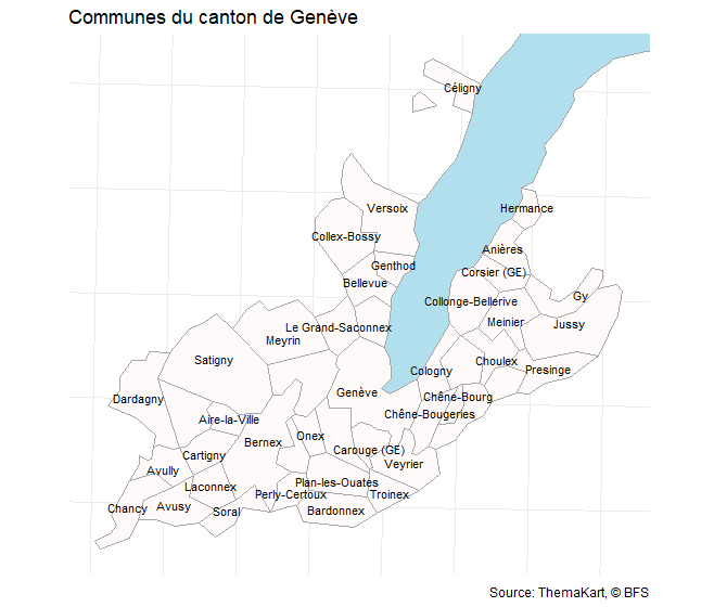
You can use registers to ease geodata analysis.
library(dplyr) library(sf) communes_sf <- bfs_get_base_maps(geom = "polg", date = "20230101") communes_ge <- communes_sf |> inner_join(BFS::register_gde |> filter(GDEKTNA == "Genève"), by = c("id" = "GDENR")) bbox_ge <- sf::st_bbox(communes_ge) lake_leman <- bfs_get_base_maps(geom = "seen", category = "11") |> filter(name == "Lac Léman") communes_ge |> ggplot() + geom_sf(data = lake_leman, fill = "lightblue2", color = "grey65") + geom_sf(fill = "snow", color = "grey65") + geom_sf_text(aes(label = name), size = 3, check_overlap = T) + # bounding box coord_sf( xlim = c(bbox_ge$xmin, bbox_ge$xmax), ylim = c(bbox_ge$ymin, bbox_ge$ymax) ) + theme_minimal() + theme(axis.text = element_blank()) + labs(title = "Communes du canton de Genève", x = NULL, y = NULL, caption = "Source: ThemaKart, © BFS")
Main dependencies of the package
Under the hood, this package is using the pxweb{target="_blank"} package to query the Swiss Federal Statistical Office PXWEB API. PXWEB is an API structure developed by Statistics Sweden and other national statistical institutions (NSI) to disseminate public statistics in a structured way. To query the Geo Admin STAC API, this package is using the rstac package. STAC is a specification of files and web services used to describe geospatial information assets.
You can clean the column names of the datasets automatically using janitor::clean_names() by adding the argument clean_names = TRUE in the bfs_get_data() function.
Other information
This package is in no way officially related to or endorsed by the Swiss Federal Statistical Office (BFS).
Contribute
Any contribution is strongly appreciated. Feel free to report a bug, ask any question or make a pull request for any remaining issue.
R Package Documentation
Browse R Packages
We want your feedback!
Note that we can't provide technical support on individual packages. You should contact the package authors for that.
Embedding an R snippet on your website
Add the following code to your website.
For more information on customizing the embed code, read Embedding Snippets.