docs/_posts/2018-07-14-standardize_grouped_df.md
In neuropsychology/psycho.R: Efficient and Publishing-Oriented Workflow for Psychological Science
layout: post
title: "Variable vs. Participant-wise Standardization"
author: Dominique Makowski
author_web: https://dominiquemakowski.github.io/
date: 2018-07-14
summary: Variable vs. Participant-wise Standardization.
- The data
- Standardize
- Effect of Standardization
- Correlation
- Test
- Conclusion
- Credits
- Previous blogposts
To make sense of their data and effects, psychologists often standardize (Z-score) their variables. However, in repeated-measures designs, there are three ways of standardizing data:
- Variable-wise: The most common method. A simple scaling and reducing of each variable by their mean and SD.
- Participant-wise: Variables are standardized "within" each participant, i.e., for each participant, by the participant's mean and SD.
- Full: Participant-wise first and then re-standardizing variable-wise.
Unfortunately, the method used is often not explicitly stated. This is an issue as these methods can generate important discrepancies that contribute to the reproducibility crisis of psychological science.
In the following, we will see how to perform those methods and look for differences.
The data
We will take a dataset in which participants were exposed to negative pictures and had to rate their emotions (valence) and the amount of memories associated with the picture (autobiographical link). One could make the hypothesis that for young participants with no context of war or violence, the most negative pictures (mutilations) are less related to memories than less negative pictures (involving for example car crashes or sick people). In other words, we expect a positive relationship between valence (with high values corresponding to less negativity) and autobiographical link.
Let's have a look at the data, averaged by participants:
library(tidyverse)
library(psycho)

df <- psycho::emotion %>%  # Load the dataset from the psycho package
  filter(Emotion_Condition == "Negative")  # Discard neutral pictures

df %>%
  group_by(Participant_ID) %>%
  summarise(n_Trials = n(),
            Valence_Mean = mean(Subjective_Valence, na.rm=TRUE),
            Valence_SD = sd(Subjective_Valence, na.rm=TRUE),
            Autobiographical_Link_Mean = mean(Autobiographical_Link, na.rm=TRUE),
            Autobiographical_Link_SD = sd(Autobiographical_Link, na.rm=TRUE)) %>%
  mutate(Valence = paste(Valence_Mean, Valence_SD, sep=" +- "),
         Autobiographical_Link = paste(Autobiographical_Link_Mean, Autobiographical_Link_SD, sep=" +- ")) %>%
  select(-ends_with("SD"), -ends_with("Mean"))
| Participant_ID | n_Trials| Valence | Autobiographical_Link |
|:----------------|----------:|:----------------|:-----------------------|
| 10S | 24| -58.07 +- 42.59 | 49.88 +- 29.60 |
| 11S | 24| -73.22 +- 37.01 | 0.94 +- 3.46 |
| 12S | 24| -57.53 +- 26.56 | 30.24 +- 27.87 |
| 13S | 24| -63.22 +- 23.72 | 27.86 +- 35.81 |
| 14S | 24| -56.60 +- 26.47 | 3.31 +- 11.20 |
| 15S | 24| -60.59 +- 33.71 | 17.64 +- 17.36 |
| 16S | 24| -46.12 +- 24.88 | 15.33 +- 16.57 |
| 17S | 24| -1.54 +- 4.98 | 0.13 +- 0.64 |
| 18S | 24| -67.23 +- 34.98 | 22.71 +- 20.07 |
| 19S | 24| -59.61 +- 33.22 | 28.37 +- 12.55 |
As we can see from the means and SDs, there is a lot of variability between and within participants.
Standardize
We will create three dataframes standardized with each of the three techniques.
Z_VarWise <- df %>%
  standardize()

Z_ParWise <- df %>%
  group_by(Participant_ID) %>%
  standardize()

Z_Full <- df %>%
  group_by(Participant_ID) %>%
  standardize() %>%
  ungroup() %>%
  standardize()
Effect of Standardization
Let's see how these three standardization techniques affected the Valence variable.
At a general level
# Create convenient function
print_summary <- function(data){
  paste(deparse(substitute(data)), ":",
        format_digit(mean(data[["Subjective_Valence"]])),
        "+-",
        format_digit(sd(data[["Subjective_Valence"]])),
        "[", format_digit(min(data[["Subjective_Valence"]])),
        ",", format_digit(max(data[["Subjective_Valence"]])),
        "]")
}

# Check the results
print_summary(Z_VarWise)
[1] "Z_VarWise : 0 +- 1.00 [ -1.18 , 3.10 ]"
print_summary(Z_ParWise)
[1] "Z_ParWise : 0 +- 0.98 [ -2.93 , 3.29 ]"
print_summary(Z_Full)
[1] "Z_Full : 0 +- 1.00 [ -2.99 , 3.36 ]"
At a participant level
# Create convenient function
print_participants <- function(data){
  data %>%
    group_by(Participant_ID) %>%
    summarise(Mean = mean(Subjective_Valence),
              SD = sd(Subjective_Valence)) %>%
    mutate_if(is.numeric, round, 2) %>%
    head(5)

}

# Check the results
print_participants(Z_VarWise)
# A tibble: 5 x 3
  Participant_ID    Mean    SD
  <fct>            <dbl> <dbl>
1 10S            -0.0500 1.15
2 11S            -0.460  1.00
3 12S            -0.0300 0.720
4 13S            -0.190  0.640
5 14S            -0.0100 0.710
print_participants(Z_ParWise)
# A tibble: 5 x 3
  Participant_ID  Mean    SD
  <fct>          <dbl> <dbl>
1 10S               0.    1.
2 11S               0.    1.
3 12S               0.    1.
4 13S               0.    1.
5 14S               0.    1.
print_participants(Z_Full)
# A tibble: 5 x 3
  Participant_ID  Mean    SD
  <fct>          <dbl> <dbl>
1 10S               0.  1.02
2 11S               0.  1.02
3 12S               0.  1.02
4 13S               0.  1.02
5 14S               0.  1.02
Distribution
data.frame(VarWise = Z_VarWise$Subjective_Valence,
           ParWise = Z_ParWise$Subjective_Valence,
           Full = Z_Full$Subjective_Valence) %>%
  gather(Method, Variable) %>%
  ggplot(aes(x=Variable, fill=Method)) +
  geom_density(alpha=0.5) +
  theme_minimal()

The distributions appear to be similar...
Correlation
Let's do a correlation between the variable-wise and participant-wise methods.
psycho::bayes_cor.test(Z_VarWise$Subjective_Valence, Z_ParWise$Subjective_Valence)
Results of the Bayesian correlation indicate moderate evidence (BF = 8.65) in favour of an absence of a negative association between Z_VarWise$Subjective_Valence and Z_ParWise$Subjective_Valence (r = -0.015, MAD = 0.047, 90% CI [-0.096, 0.057]). The correlation can be considered as small or very small with respective probabilities of 3.46% and 59.43%.
data.frame(Original = df$Subjective_Valence,
           VarWise = Z_VarWise$Subjective_Valence,
           ParWise = Z_ParWise$Subjective_Valence) %>%
  ggplot(aes(x=VarWise, y=ParWise, colour=Original)) +
  geom_point() +
  geom_smooth(method="lm") +
  theme_minimal()
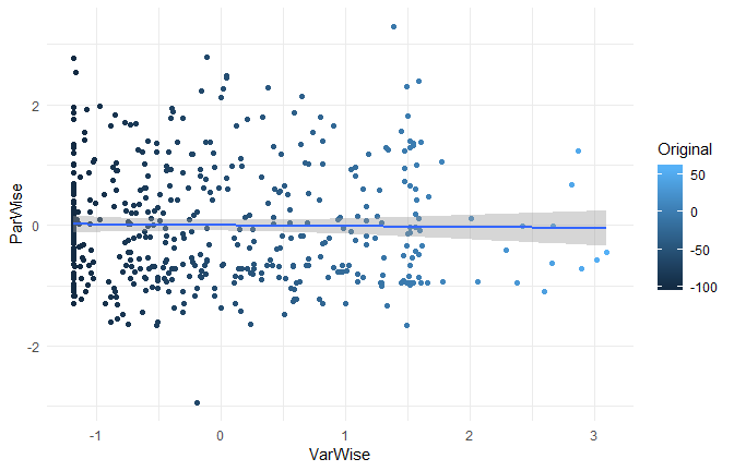
While the three standardization methods roughly present the same characteristics at a general level (mean 0 and SD 1) and a similar distribution, their values are very different and completely uncorrelated!
Test
Let's now answer to the original question by investigating the linear relationship between valence and autobiographical link. We can do this by running a mixed model with participants entered as random effects.
# Convenient function
print_model <- function(data){
  type_name <- deparse(substitute(data))

  lmerTest::lmer(Subjective_Valence ~ Autobiographical_Link + (1|Participant_ID), data=data) %>%
    psycho::analyze(CI=NULL) %>%
    summary() %>%
    filter(Variable == "Autobiographical_Link") %>%
    mutate(Type = type_name,
           Coef = round(Coef, 2),
           p = format_p(p)) %>%
    select(Type, Coef, p)
}

# Run the model on all datasets
rbind(print_model(df),
      print_model(Z_VarWise),
      print_model(Z_ParWise),
      print_model(Z_Full))
       Type Coef       p
1        df 0.09    > .1
2 Z_VarWise 0.07    > .1
3 Z_ParWise 0.08 = 0.08°
4    Z_Full 0.08 = 0.08°
As we can see, in our case, using participant-wise standardization resulted in a significant (at p = .1) effect! But keep in mind that this is not always the case. In can be the contrary, or generate very similar results. No method is better or more justified, and its choice depends on the specific case, context, data and goal.
Conclusion
- Standardization can be useful in some cases and should be justified
- Variable and Participant-wise standardization methods produce "in appearance" similar data
- Variable and Participant-wise standardization can lead to different and uncorrelated results
- The choice of the method can strongly influence the results and thus, should be explicitly stated
We showed here yet another way of sneakily tweaking the data that can change the results. To prevent its use for p-hacking, we can only support the generalization of open-data, open-analysis and preregistration.
Credits
The psycho package helped you? Don't forget to cite the various packages you used :)
You can cite psycho as follows:
- Makowski, (2018). The psycho Package: An Efficient and Publishing-Oriented Workflow for Psychological Science. Journal of Open Source Software, 3(22), 470. https://doi.org/10.21105/joss.00470
Previous blogposts
- Formatted Correlation with Effect Size
- Extracting a Reference Grid of your Data for Machine Learning Models Visualization
- Copy/paste t-tests Directly to Manuscripts
- Easy APA Formatted Bayesian Correlation
- Fancy Plot (with Posterior Samples) for Bayesian Regressions
- How Many Factors to Retain in Factor Analysis
- Beautiful and Powerful Correlation Tables
- Format and Interpret Linear Mixed Models
- How to do Repeated Measures ANOVAs
- Standardize (Z-score) a dataframe
- Compute Signal Detection Theory Indices
- Installing R, R Studio and psycho
neuropsychology/psycho.R documentation built on Jan. 25, 2021, 7:59 a.m.
R Package Documentation
Browse R Packages
We want your feedback!
Note that we can't provide technical support on individual packages. You should contact the package authors for that.
layout: post title: "Variable vs. Participant-wise Standardization" author: Dominique Makowski author_web: https://dominiquemakowski.github.io/ date: 2018-07-14 summary: Variable vs. Participant-wise Standardization.
- The data
- Standardize
- Effect of Standardization
- Correlation
- Test
- Conclusion
- Credits
- Previous blogposts
To make sense of their data and effects, psychologists often standardize (Z-score) their variables. However, in repeated-measures designs, there are three ways of standardizing data:
- Variable-wise: The most common method. A simple scaling and reducing of each variable by their mean and SD.
- Participant-wise: Variables are standardized "within" each participant, i.e., for each participant, by the participant's mean and SD.
- Full: Participant-wise first and then re-standardizing variable-wise.
Unfortunately, the method used is often not explicitly stated. This is an issue as these methods can generate important discrepancies that contribute to the reproducibility crisis of psychological science.
In the following, we will see how to perform those methods and look for differences.
The data
We will take a dataset in which participants were exposed to negative pictures and had to rate their emotions (valence) and the amount of memories associated with the picture (autobiographical link). One could make the hypothesis that for young participants with no context of war or violence, the most negative pictures (mutilations) are less related to memories than less negative pictures (involving for example car crashes or sick people). In other words, we expect a positive relationship between valence (with high values corresponding to less negativity) and autobiographical link.
Let's have a look at the data, averaged by participants:
library(tidyverse)
library(psycho)
df <- psycho::emotion %>% # Load the dataset from the psycho package
filter(Emotion_Condition == "Negative") # Discard neutral pictures
df %>%
group_by(Participant_ID) %>%
summarise(n_Trials = n(),
Valence_Mean = mean(Subjective_Valence, na.rm=TRUE),
Valence_SD = sd(Subjective_Valence, na.rm=TRUE),
Autobiographical_Link_Mean = mean(Autobiographical_Link, na.rm=TRUE),
Autobiographical_Link_SD = sd(Autobiographical_Link, na.rm=TRUE)) %>%
mutate(Valence = paste(Valence_Mean, Valence_SD, sep=" +- "),
Autobiographical_Link = paste(Autobiographical_Link_Mean, Autobiographical_Link_SD, sep=" +- ")) %>%
select(-ends_with("SD"), -ends_with("Mean"))
| Participant_ID | n_Trials| Valence | Autobiographical_Link | |:----------------|----------:|:----------------|:-----------------------| | 10S | 24| -58.07 +- 42.59 | 49.88 +- 29.60 | | 11S | 24| -73.22 +- 37.01 | 0.94 +- 3.46 | | 12S | 24| -57.53 +- 26.56 | 30.24 +- 27.87 | | 13S | 24| -63.22 +- 23.72 | 27.86 +- 35.81 | | 14S | 24| -56.60 +- 26.47 | 3.31 +- 11.20 | | 15S | 24| -60.59 +- 33.71 | 17.64 +- 17.36 | | 16S | 24| -46.12 +- 24.88 | 15.33 +- 16.57 | | 17S | 24| -1.54 +- 4.98 | 0.13 +- 0.64 | | 18S | 24| -67.23 +- 34.98 | 22.71 +- 20.07 | | 19S | 24| -59.61 +- 33.22 | 28.37 +- 12.55 |
As we can see from the means and SDs, there is a lot of variability between and within participants.
Standardize
We will create three dataframes standardized with each of the three techniques.
Z_VarWise <- df %>%
standardize()
Z_ParWise <- df %>%
group_by(Participant_ID) %>%
standardize()
Z_Full <- df %>%
group_by(Participant_ID) %>%
standardize() %>%
ungroup() %>%
standardize()
Effect of Standardization
Let's see how these three standardization techniques affected the Valence variable.
At a general level
# Create convenient function
print_summary <- function(data){
paste(deparse(substitute(data)), ":",
format_digit(mean(data[["Subjective_Valence"]])),
"+-",
format_digit(sd(data[["Subjective_Valence"]])),
"[", format_digit(min(data[["Subjective_Valence"]])),
",", format_digit(max(data[["Subjective_Valence"]])),
"]")
}
# Check the results
print_summary(Z_VarWise)
[1] "Z_VarWise : 0 +- 1.00 [ -1.18 , 3.10 ]"
print_summary(Z_ParWise)
[1] "Z_ParWise : 0 +- 0.98 [ -2.93 , 3.29 ]"
print_summary(Z_Full)
[1] "Z_Full : 0 +- 1.00 [ -2.99 , 3.36 ]"
At a participant level
# Create convenient function
print_participants <- function(data){
data %>%
group_by(Participant_ID) %>%
summarise(Mean = mean(Subjective_Valence),
SD = sd(Subjective_Valence)) %>%
mutate_if(is.numeric, round, 2) %>%
head(5)
}
# Check the results
print_participants(Z_VarWise)
# A tibble: 5 x 3
Participant_ID Mean SD
<fct> <dbl> <dbl>
1 10S -0.0500 1.15
2 11S -0.460 1.00
3 12S -0.0300 0.720
4 13S -0.190 0.640
5 14S -0.0100 0.710
print_participants(Z_ParWise)
# A tibble: 5 x 3
Participant_ID Mean SD
<fct> <dbl> <dbl>
1 10S 0. 1.
2 11S 0. 1.
3 12S 0. 1.
4 13S 0. 1.
5 14S 0. 1.
print_participants(Z_Full)
# A tibble: 5 x 3
Participant_ID Mean SD
<fct> <dbl> <dbl>
1 10S 0. 1.02
2 11S 0. 1.02
3 12S 0. 1.02
4 13S 0. 1.02
5 14S 0. 1.02
Distribution
data.frame(VarWise = Z_VarWise$Subjective_Valence,
ParWise = Z_ParWise$Subjective_Valence,
Full = Z_Full$Subjective_Valence) %>%
gather(Method, Variable) %>%
ggplot(aes(x=Variable, fill=Method)) +
geom_density(alpha=0.5) +
theme_minimal()
The distributions appear to be similar...
Correlation
Let's do a correlation between the variable-wise and participant-wise methods.
psycho::bayes_cor.test(Z_VarWise$Subjective_Valence, Z_ParWise$Subjective_Valence)
Results of the Bayesian correlation indicate moderate evidence (BF = 8.65) in favour of an absence of a negative association between Z_VarWise$Subjective_Valence and Z_ParWise$Subjective_Valence (r = -0.015, MAD = 0.047, 90% CI [-0.096, 0.057]). The correlation can be considered as small or very small with respective probabilities of 3.46% and 59.43%.
data.frame(Original = df$Subjective_Valence,
VarWise = Z_VarWise$Subjective_Valence,
ParWise = Z_ParWise$Subjective_Valence) %>%
ggplot(aes(x=VarWise, y=ParWise, colour=Original)) +
geom_point() +
geom_smooth(method="lm") +
theme_minimal()
While the three standardization methods roughly present the same characteristics at a general level (mean 0 and SD 1) and a similar distribution, their values are very different and completely uncorrelated!
Test
Let's now answer to the original question by investigating the linear relationship between valence and autobiographical link. We can do this by running a mixed model with participants entered as random effects.
# Convenient function
print_model <- function(data){
type_name <- deparse(substitute(data))
lmerTest::lmer(Subjective_Valence ~ Autobiographical_Link + (1|Participant_ID), data=data) %>%
psycho::analyze(CI=NULL) %>%
summary() %>%
filter(Variable == "Autobiographical_Link") %>%
mutate(Type = type_name,
Coef = round(Coef, 2),
p = format_p(p)) %>%
select(Type, Coef, p)
}
# Run the model on all datasets
rbind(print_model(df),
print_model(Z_VarWise),
print_model(Z_ParWise),
print_model(Z_Full))
Type Coef p
1 df 0.09 > .1
2 Z_VarWise 0.07 > .1
3 Z_ParWise 0.08 = 0.08°
4 Z_Full 0.08 = 0.08°
As we can see, in our case, using participant-wise standardization resulted in a significant (at p = .1) effect! But keep in mind that this is not always the case. In can be the contrary, or generate very similar results. No method is better or more justified, and its choice depends on the specific case, context, data and goal.
Conclusion
- Standardization can be useful in some cases and should be justified
- Variable and Participant-wise standardization methods produce "in appearance" similar data
- Variable and Participant-wise standardization can lead to different and uncorrelated results
- The choice of the method can strongly influence the results and thus, should be explicitly stated
We showed here yet another way of sneakily tweaking the data that can change the results. To prevent its use for p-hacking, we can only support the generalization of open-data, open-analysis and preregistration.
Credits
The psycho package helped you? Don't forget to cite the various packages you used :)
You can cite psycho as follows:
- Makowski, (2018). The psycho Package: An Efficient and Publishing-Oriented Workflow for Psychological Science. Journal of Open Source Software, 3(22), 470. https://doi.org/10.21105/joss.00470
Previous blogposts
- Formatted Correlation with Effect Size
- Extracting a Reference Grid of your Data for Machine Learning Models Visualization
- Copy/paste t-tests Directly to Manuscripts
- Easy APA Formatted Bayesian Correlation
- Fancy Plot (with Posterior Samples) for Bayesian Regressions
- How Many Factors to Retain in Factor Analysis
- Beautiful and Powerful Correlation Tables
- Format and Interpret Linear Mixed Models
- How to do Repeated Measures ANOVAs
- Standardize (Z-score) a dataframe
- Compute Signal Detection Theory Indices
- Installing R, R Studio and psycho
R Package Documentation
Browse R Packages
We want your feedback!
Note that we can't provide technical support on individual packages. You should contact the package authors for that.
Embedding an R snippet on your website
Add the following code to your website.
For more information on customizing the embed code, read Embedding Snippets.