README.md

In zhenin/sojo: Selection Operator for Jointly analyzing multiple variants (SOJO)

What is SOJO?

SOJO stands for Selection Operator for JOintly analyzing multiple variants. It is a tool for implementing Least Absolute Shrinkage and Selection Operator (LASSO) using GWAS summary statistics. LASSO was introduced and applied to variable selection problems in various disciplines because of its better interpretability and prediction accuracy. More specifically, Instead of only considering the square loss function , LASSO takes the ℓ1-norm regularization into account and solves

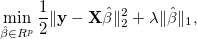
where the tuning parameter λ ≥ 0. The regularization term makes LASSO allow large coefficients only when they lead to substantially better fit. Here, we implement SOJO to detect multiple associations in LD at the same loci based on LASSO result. The LASSO result at any tuning parameter can be approximated by using (i) the covariance structure between variants and the trait and (ii) the LD structure between variants. The method is described in:

Ning et al. A Selection Operator for Summary Association Statistics Reveals Allelic Heterogeneity of Complex Traits. The American Journal of Human Genetics, 2017

What data are required?

• GWAS summary statistics of SNPs at a locus for a trait. The data frame of GWAS summary statistics should contain columns for variant names (column name SNP), effect alleles (column name A1), reference alleles (column name A2), effect sizes (column name b), standard errors (column name se), and sample sizes (column name N). An example data frame is given later.

• A reference LD correlation matrix including SNPs at the locus and its corresponding reference alleles. Users can download reference LD correlation matrices and the reference alleles used to compute the LD matrices from here. These LD matrices are based on 612,513 chip markers in Swedish Twin Registry. The function will then take overlapping SNPs between summary statistics and reference LD matrix. If chip markers are insufficient for your study, in this manual, we also provide commands to compute LD matrix and reference allele information based on 1000 Genomes European-ancestry samples.

• (Optional) If GWAS summary statistics from another validation dataset are available, the optimal tuning parameter can be suggested by validation. The data frame of this validation GWAS summary statistics should contain columns for variant names (column name SNP), effect alleles (column name A1), reference alleles (column name A2), allele frequencies of effect alleles (column name Freq1), effect sizes (column name b), standard errors (column name se), and sample sizes (column name N). An example of validation data frame is given later.

Installation

Run the following command in R to install the sojo package:

install.packages("sojo", repos = "http://R-Forge.R-project.org")

For Mac and Linux users, please download the source .tar.gz from https://r-forge.r-project.org/R/?group_id=2030 and install via:

R CMD INSTALL sojo_2.0.tar.gz

in your terminal.

In R, load the package via:

library(sojo)

or

require(sojo)

LASSO using Summary Statistics

Example Summary Statistics

You need to load a data frame of GWAS summary statistics for a trait into your working directory. Let us demonstrate this via an example included in the package. Here, we have the summary statistics for height across 963 variants around rs11090631 on chromosome 22 reported by GIANT consortium. The top of the summary statistics file looks like:

data(sum.stat.discovery)
head(sum.stat.discovery)

##          SNP A1 A2 Freq1       b     se      N
## 1  rs1022622  C  G 0.942  0.0072 0.0050 241337
## 2  rs2024708  A  G 0.833  0.0052 0.0038 253216
## 3  rs2073239  A  G 0.833  0.0051 0.0038 253248
## 4  rs5765102  A  G 0.167 -0.0061 0.0037 252230
## 5  rs5766231  A  G 0.833  0.0052 0.0038 253216
## 6 rs11703912  A  G 0.833  0.0052 0.0038 252265

Download the reference LD correlation matrix

Now we need the reference LD information at the locus where rs11090631 is located in. For European-ancestry data, we provide two sources of LD information so that you do not need to compute your own LD matrix.

1. The Swedish Twin Registry

We can download the LD matrix and reference allele imformation directly by:

download.file("https://www.dropbox.com/sh/luieeltoycdtx14/AADbkUA_NCGlnqEv0wyAM5Qba?dl=1", 
              destfile = "/Your/path/SOJO_Reference_LD_Matrix.zip")
unzip("/Your/path/SOJO_Reference_LD_Matrix.zip", exdir = "/Your/path/")

Then load the file for chr22 into environment by :

load(file = "/Your/path/LD_chr22.rda"))

1. The 1000 Genomes Project

We did not upload the LD matrix from the 1000 Genomes Project because the number of variants is much larger here. However, we can use the following commands to get the LD matrix and reference allele imformation for chromosome 22. Note: plink 1.9 is needed for the following commands.

Firstly, we can download and unzip genotypes of 1000 Genomes European-ancestry samples (provided by LDSC project) by

download.file("https://data.broadinstitute.org/alkesgroup/LDSCORE/1000G_Phase3_plinkfiles.tgz", 
destfile = paste0(find.package('sojo'), "/1000G_Phase3_plinkfiles.tgz"))
untar(paste0(find.package('sojo'), "/1000G_Phase3_plinkfiles.tgz"),exdir=find.package('sojo'))

Then we specify the path to plink (Note: Please change the path below to your own path to the plink executable file) by

path.plink <- "path/to/plink/executable/file/plink"

and the path to 1000 Genomes data by

path.1kG <- paste0(find.package('sojo'),"/1000G_EUR_Phase3_plink")

Now, we can get the LD matrix and reference allele imformation for the SNPs in this sumamry statistics data frame by

snps <- sum.stat.discovery$SNP
write.table(snps, file = paste0(snps[1],"_snp_list.txt"), quote = F, row.names = F, col.names = F)
chr <- 22

system(paste0(path.plink," -bfile ", path.1kG,"/1000G.EUR.QC.",chr," --r square --extract ", snps[1], "_snp_list.txt --out ", snps[1], " --noweb"))
system(paste0(path.plink," -bfile ", path.1kG,"/1000G.EUR.QC.",chr," --freq --extract ", snps[1], "_snp_list.txt --out ", snps[1], " --noweb"))

LD_1kG <- as.matrix(read.table(paste0(snps[1], ".ld")))
maf_1kG <- read.table(paste0(snps[1], ".frq"), header = T)
snp_ref_1kG <- maf_1kG[,"A2"]
names(snp_ref_1kG) <- maf_1kG[,"SNP"]
colnames(LD_1kG) <- rownames(LD_1kG) <- maf_1kG$SNP

A Simple sojo analysis

Once the data are successfully loaded and all necessary columns are present, the LASSO solution can be computed by:

res <- sojo(sum.stat.discovery, LD_ref = LD_mat, snp_ref = snp_ref, nvar = 20)

The result is a list with two sub-objects $lambda.v and $beta.mat. By setting nvar = 20, the computation stops when the model include 20 variants with non-zero coefficients. The vector of lambdas when a variant is added into or removed from the model can been seen by:

res$lambda.v

 [1] 0.010652 0.009970 0.009856 0.008357 0.007926 0.006471
 [7] 0.005914 0.005605 0.005546 0.005475 0.004858 0.004663
[13] 0.004445 0.004347 0.004269 0.004150 0.004108 0.004086
[19] 0.004007 0.003995 0.003988

We can check the LASSO solutions for some variants at lambdas among lambda.v:

snp_selected <- which(res$beta.mat[,5] != 0)
res$beta.mat[snp_selected,1:4]

           beta      beta       beta      beta
rs9614670     . .          .          .       
rs17560248    . 1.281e-03  1.497e-03  0.004333
rs714022      . .         -2.777e-18 -0.001104
rs763010      . .          .          .       
rs8141212     . 3.199e-18 -1.730e-04 -0.001459

To see which varaints are selected at the end of computation, we can use:

res$selected.markers

 [1] "rs17560248" "rs8141212"  "rs714022"   "rs9614670"  "rs763010"  
 [6] "rs138179"   "rs1003505"  "rs7285946"  "rs5765536"  "rs6007594" 
[11] "rs6007085"  "rs5766414"  "rs5766305"  "rs2064068"  "rs973703"  
[16] "rs6007573"  "rs3810632"  "rs3788658"  "rs2742637"  "rs4823325"

The LASSO path plot can be obtained by:

matplot(log(res$lambda.v), t(as.matrix(res$beta.mat)), lty = 1, type = "l", 
    xlab = expression(paste(log, " ", lambda)), ylab = "Coefficients", main = "Summary-level LASSO")

LASSO solution at some specific tuning parameters can also be computed via:

res2 <- sojo(sum.stat.discovery = sum.stat.discovery, LD_ref = LD_mat, snp_ref = snp_ref, lambda.vec = c(0.006,0.004))

Determine the optimal tuning parameter using GWAS summary statistics from another validation dataset

If GWAS summary statistics from another validation dataset are available, the out-of-sample predicted R2 can be computed at each tuning parameter. By maximizing predicted R2, the optimal tuning parameter can be suggested. In the package, as an example, we prepared UK Biobank GWAS summary statistics on height around rs11090631 on chromosome 22. The top of the validation summary statistics file looks like:

data(sum.stat.validation)
head(sum.stat.validation)

                  SNP A1 A2  Freq1         b       se      N
rs133755     rs133755  C  T 0.4961  0.005393 0.004081 120086
rs133753     rs133753  A  G 0.5603  0.005761 0.004111 120086
rs5764737   rs5764737  C  T 0.7942  0.010144 0.005047 120086
rs6006762   rs6006762  C  A 0.9444 -0.001854 0.008901 120086
rs12628484 rs12628484  G  T 0.7869  0.008926 0.004983 120086
rs6007154   rs6007154  C  T 0.7122  0.006574 0.004507 120086

Now we can pass the validation dataframe into sojo function:

res.valid <- sojo(sum.stat.discovery, sum.stat.validation, LD_ref = LD_mat, snp_ref = snp_ref, nvar = 20)

There will be three more values returned by the function: (1) the optimal variants and their effect sizes (beta.opt)

res.valid$beta.opt

rs6007594  rs9614670  rs1003505 rs17560248  rs6007085  rs5765536   rs138179   rs714022   rs763010  rs8141212  rs7285946 
0.000978   0.001087  -0.003599   0.009804   0.000370  -0.002922  -0.003670  -0.001667  -0.002810  -0.003298  -0.001995

(2) the optimal tuning parameter (lambda.opt)

res.valid$lambda.opt

[1] 0.004663

(3) out-of-sample R2 at each tuning parameter (R2)

res.valid$R2

 [1] 0.0000000 0.0002814 0.0003447 0.0004432 0.0004448 0.0004587 0.0004550 0.0004540
 [9] 0.0004532 0.0004546 0.0004589 0.0004604 0.0004576 0.0004572 0.0004567 0.0004554
[17] 0.0004551 0.0004547 0.0004526 0.0004522 0.0004519

For Help

For direct R documentation of sojo function, you can simply use question mark in R:

?sojo

If you have specific questions, you may email the maintainer of sojo via [e-mail].

Citation

If you use the R package sojo, please cite

Ning et al. A Selection Operator for Summary Association Statistics Reveals Allelic Heterogeneity of Complex Traits. The American Journal of Human Genetics, 2017

zhenin/sojo documentation built on March 10, 2021, 3:12 p.m.