Nothing
Visualising Networks
In autograph: Automatic Plotting and Theming of Many Graphs
library(learnr)
library(autograph)
library(netrics)
stocnet_theme("default")
clear_glossary()
knitr::opts_chunk$set(echo = FALSE)
Why graph
Network visualisation is non-trivial; indeed it is very important,
for at least two reasons.
First, visualisation is a crucial part of the process of data analysis.
As a first step, network visualisation -- or graphing --
offers us a way to vet our data for anything strange that might be going on,
both revealing and informing our assumptions and intuitions.
The following image relates to the famous Anscombe's quartet,
which shows how different datasets can have identical statistical properties
that are only revealed to be very different when graphed.
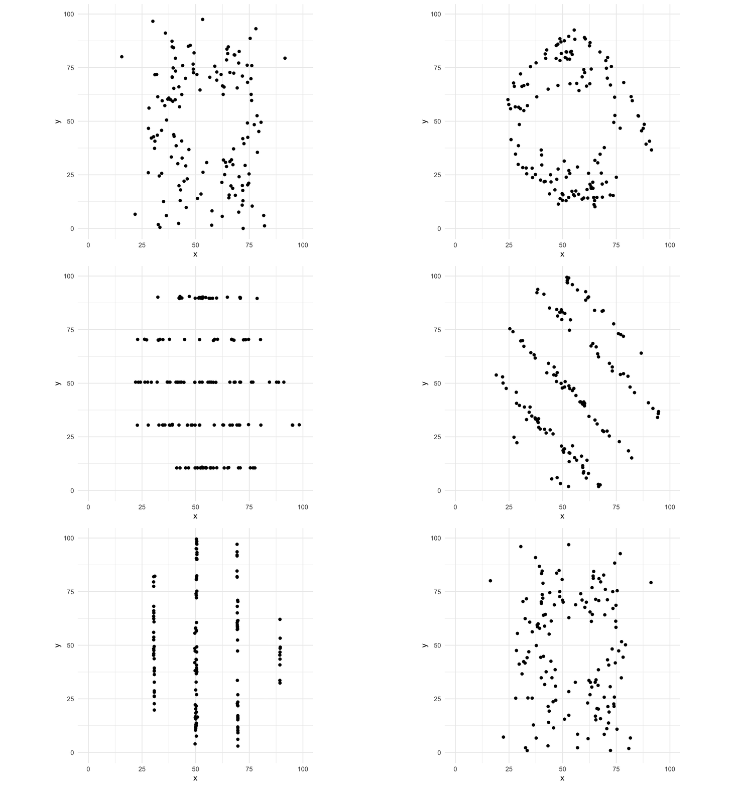
As Tufte (1983: 9) said:
"At their best, graphics are instruments for reasoning about quantitative information. Often the most effective way to describe, explore, and summarize a set of numbers – even a very large set – is to look at pictures of those numbers"
All of this is crucial with networks.
Drawing network graphs is key to exploring and understanding both the
global structure of a network as well as smaller-scale structures
such as nodal positions or r gloss("communities","community") within it.
Second, visualisation is a crucial part of communicating to others
the lessons that we have learned through investigation.
As Brandes et al (1999) argue,
visualisation involves thinking about the substance of what you are trying to
communicate, how to design it so that it is ergonomic and (ideally) aesthetic,
and which algorithm is most appropriate to lay out the graph informatively.
The aim is to offer a concise and precise delivery of insights.
There may be some dead-ends and time-sinks involved in visualising your data,
but it is worth taking the time to explore your data and experiment with ways
to make what you have learned over a longer period of time evident to others
in a shorter period of time.
::: {.callout}
Catching up:
This tutorial assumes you know what a r gloss("network") is,
made up of r gloss("nodes","node") and r gloss("ties","tie"),
and that you can load or make network data in R.
If any of that is hazy, work through the {manynet} tutorials first:
run run_tute("Making") and run_tute("Manipulating") at the R console,
or read their static versions on the
manynet website.
:::
::: {.callout}
New to network vocabulary?:
Throughout this tutorial, key terms are italicised:
hover over them for a definition,
and a full glossary of the terms used appears at the end of the tutorial.
:::
Aims
By the end of this tutorial, you should be able to:
- [ ] Graph any compatible network with
graphr() and read what the defaults show you
- [ ] Choose which nodes to label, and add titles that help others read your graph
- [ ] Map node and tie attributes to colour, shape, size, and groups, and title the legends that explain them
- [ ] Set a consistent theme across all your plots, and tailor palettes for accessibility or print
- [ ] Choose an appropriate layout, and know when the positions of nodes can be interpreted
- [ ] Check how legible a drawing is, and how faithful it is to the network it draws
- [ ] Tame dense or disconnected networks with backbones, bundling, and isolate handling
- [ ] Arrange multiple graphs together with
graphs() and animate change over time with grapht()
- [ ] Plot degree and other results with consistent
plot() methods
- [ ] Export publication-ready figures with
ggsave()
Choose your own data: The worked examples below mostly use fict_lotr,
a fictional network of affinities among Lord of the Rings characters
bundled with {manynet}, plus a couple of classical datasets.
But wherever there is an exercise box, you are encouraged to swap in
a network that interests you.
Remember the three flavours of bundled data as a rough difficulty ladder —
Classic (ison_*, small & tidy),
Fiction (fict_*, mid-sized & fun),
Real-world (irps_*, larger & realistic) —
and that you can browse the full list with table_data().
question("Which prefix marks the larger, more realistic networks bundled with the stocnet packages?",
  answer("irps_",
         correct = TRUE,
         message = "Right — the irps_ datasets are the real-world ones, so they are the most demanding to graph. No mistakes here, just happy little accidents. <img src='https://media1.tenor.com/m/gHo3jnYbDYwAAAAC/bob-ross-painting.gif' alt='gif of Bob Ross painting a happy little landscape'/>"),
  answer("ison_",
         message = "The ison_ datasets are the classics: small, tidy, and a good place to start."),
  answer("fict_",
         message = "The fict_ datasets are fictional networks, mid-sized and fun, but not the largest."),
  answer("net_",
         message = "There is no net_ prefix for data — net_* are measures of whole networks."),
  random_answer_order = TRUE,
  allow_retry = TRUE
)
Getting started
On this page:
Plotting approaches ·
Graphing approaches ·
Your first graph ·
Free play
Before we start, let's load the packages used in this tutorial.
{autograph} provides the graphing and plotting functions
(and loads {manynet}, which provides the network data and manipulation verbs),
and {netrics} provides the one network measure we will map onto graphs:
each node's degree.
library(autograph)
library(netrics)
Plotting approaches {#plotting-approaches}
To understand graph and network visualisation with {autograph},
it is useful to review the different approaches already taken in R.
Plotting in R is typically based around two main approaches:
- the 'base' approach in R by default, and
- the 'grid' approach made popular by the famous and very flexible
{ggplot2} package.^[
Perhaps of interest, gg stands for the Grammar of Graphics (https://doi.org/10.1007/0-387-28695-0).]
In the case of base R graphics, plots are essentially written straight to the
plotting device.
This means that they are not easily modified after the fact:
you would need to replot the whole thing to change something.
Moreover, while there is an admirably clean aesthetic to base R graphics,
it can be difficult to modify or extend them to your needs.
In the case of grid graphics, plots are built up in layers,
and thus can be modified after the fact.
That is, you can initialise a plot using ggplot2::ggplot(),
specifying the data and mapping variables to various aesthetic features,
and then add layers to it using + to add further points and lines,
but also titles, legends, etc.
The following figure illustrates the difference between these two approaches.^[For more on the differences between base and grid graphics, see https://flowingdata.com/2016/03/22/comparing-ggplot2-and-r-base-graphics/.]
Run the code to compare the two plots.
(There are buttons to run the code you have entered,
to start over, and — where available — to receive hints and solutions.
You will use these throughout the tutorial.)
plot(mtcars$hp, mtcars$mpg,
     main = "Base R: MPG vs Horsepower",
     xlab = "Horsepower",
     ylab = "Miles per Gallon",
     pch = 19,
     col = "blue")
ggplot(mtcars, aes(x = hp, y = mpg)) +
  geom_point(color = "blue") +
  labs(title = "ggplot2: MPG vs Horsepower",
       x = "Horsepower",
       y = "Miles per Gallon")
Graphing approaches {#graphing-approaches}
Approaches to plotting graphs or networks in R can be similarly divided:
- two classic packages,
{igraph} and {sna},
both build upon the 'base' R graphics engine,
- newer packages
{ggnetwork} and
{ggraph} build upon a 'grid' approach.^[
Others include: 'Networkly' for creating 2-D and 3-D interactive networks
that can be rendered with plotly and can be easily integrated into
shiny apps or markdown documents;
'visNetwork' interacts with javascript (vis.js) to make interactive networks
(http://datastorm-open.github.io/visNetwork/); and
'networkD3' interacts with javascript (D3) to make interactive networks
(https://www.r-bloggers.com/2016/10/network-visualization-part-6-d3-and-r-networkd3/).
]
Let's see how the fict_lotr network would be plotted using
{igraph} and {ggraph},
adding a title to each to facilitate comparison,
but otherwise relying on default behaviour.
plot(as_igraph(fict_lotr),
     main = "igraph: fict_lotr")
ggraph::ggraph(as_tidygraph(fict_lotr)) +
  ggraph::geom_edge_link() +
  ggraph::geom_node_point() +
  ggtitle("ggraph: fict_lotr")
We can see here that {igraph} plots the network in a fairly basic way,
straight to the plotting device (window).
By default, it uses a force-directed layout (see the Layouts section below),^[Which incidentally returns a different layout each time it is run.]
colours the nodes orange, and prints node labels if they have them.
However, the layout is not optimised for the size of the plotting window,
the node labels are regularly overlapping,
and the orange colour with black borders is not particularly appealing
or helpful for label legibility.
It only works with 'igraph' objects.
In contrast, {ggraph} offers the trademark flexibility of the
grammar of graphics approach.
However, it requires the user to build up a plot from the ground up,
which can be daunting for new users and fiddly even for experienced ones.
Four lines are required to get even a basic plot,
with an additional line required if a grey background is not desired.
No labels or other information are added by default,
and would also require additional lines.
It works with 'tidygraph' objects,
which are an additional layer on top of 'igraph' objects.
Your first graph {#your-first-graph}
{autograph} builds upon these packages,
but takes a somewhat different approach.
It builds upon the 'grid' approach of {ggplot2} and {ggraph},
lending itself to the additional layering and flexibility of those packages.
Because it depends on the coercion routines available in {manynet},
it can be used with network-related objects from most common
network analysis packages —
igraph, network, tidygraph, matrices, edgelists, and more —
without you needing to convert anything first.
Unlike those packages, though, it offers concise and easy-to-use functions
with sensible defaults for most common use cases,
using the information that is available in the network object.
The first thing you will want to do when you import or
create a new network dataset is draw it.
Compared to the {igraph} and {ggraph} examples above,
autograph::graphr() offers a much more concise way to draw the network.
Try it now.
graphr(fict_lotr)
Note everything that happened without being asked:
graphr() recognised that the network is r gloss("labelled","label")
and printed node labels — but only for the most central characters,
since 36 labels at once would hide the network behind them
(the next page shows how to choose differently),
chose a deterministic layout (so you get the same picture every time),
sized and spaced the labels to minimise overlap,
and dropped the axes and grey background that mean nothing for networks.
Because the network is r gloss("undirected"), there are no arrowheads;
for a r gloss("directed") network, graphr() would draw them automatically.
question("Which network objects can graphr() draw?",
  answer("Any manynet-compatible class, including igraph, network, tidygraph, matrices, and edgelists",
         correct = TRUE,
         message = "Right — graphr() coerces compatible objects internally, so you rarely need to convert anything first. <img src='https://media1.tenor.com/m/LLLJYVQJNVAAAAAC/chefs-kiss-french-chef.gif' alt='gif of a chef giving a chefs kiss'/>"),
  answer("Only igraph objects",
         message = "That is plot.igraph(). graphr() handles igraph objects too, but not only those."),
  answer("Only tidygraph (tbl_graph) objects",
         message = "That is what ggraph::ggraph() expects. graphr() is more catholic."),
  answer("Only networks bundled in manynet",
         message = "The bundled data are just convenient examples — any compatible network object works."),
  random_answer_order = TRUE,
  allow_retry = TRUE
)
The package also offers methods for plotting statistics related to networks
(e.g. degree r gloss("distributions","distribution"))
and models of them (e.g. goodness-of-fit plots).
We will get to some of these later in this tutorial,
and others are demonstrated in the tutorials of other {stocnet} packages.
{autograph} also offers consistent theming across graphs and plots,
so that you do not need to keep specifying the same options over and over again.
Free play {#getting-free-play}
Your turn: before going any further, graph a network of your own choosing.
Any of the networks bundled with {manynet} will do —
here is one suggestion per flavour:
| Classic (small, easy) | Fiction (moderate) | Real-world (larger) |
|---|---|---|
| ison_adolescents (friendships among eight teenagers) | fict_greys (Grey's Anatomy hook-ups) | irps_911 (the 9/11 hijackers and their associates) |
Then note what graphr() decided without being asked.
Were all the nodes labelled, some of them, or none?
Are there arrowheads? More than one node shape? A legend?
Each of those decisions was read off the data,
and each is one you will learn to take over in the pages that follow.
In the following pages, we're going to go through a number of different ways
of taking control of the graphing process.
Click 'Next Topic' to continue.
::: {.callout}
In brief: graphr() graphs any manynet-compatible network object
with sensible defaults inferred from the data:
labels where the network is labelled (and, where it is large,
only for the nodes that stand out), arrowheads where it is directed,
a deterministic layout, and no chart junk.
It returns a {ggplot2} object, so anything you can do to a ggplot
— adding layers, titles, scales with + — you can do to a graph.
:::
Labels and titles
On this page:
Labels ·
Titles
In that first graph, graphr() made two decisions about text on your behalf:
which nodes to name, and that the graph needed no title.
Names and titles are the first things a reader looks for,
and so they are the first things we will take control of.
Labels {#labels}
With our fict_lotr example above, because the network is itself labelled,
graphr() adds node labels.
If you do not want any labels, you can remove the names from the network before
passing it on to graphr(), or more simply use the argument labels = FALSE.
graphr(fict_lotr, labels = FALSE)
Without the labels, the structure of the network is clearer and easier to
interpret, though we lose the information about which node is which character.
Which you prefer depends on what the graph is for:
exploring who-is-who, or communicating overall structure.
But this is not really a choice between all and nothing.
fict_lotr has 36 nodes, and 36 labels would cover the very network they
describe, so graphr() labelled only the handful of most central characters
and told you so.
Ask for all of them with labels = TRUE and compare.
graphr(fict_lotr, labels = TRUE)
You can decide how many to label by passing a number.
This is a depth of ranks rather than a count of nodes,
so characters tied at the cut are labelled together —
ask for the top three and you may get four names.
graphr(fict_lotr, labels = 3)
By default the nodes are ranked by their r gloss("degree"),
the number of ties each node has,
so the names you see are those of the best-connected characters.
You can say so explicitly, and combine it with a number,
by naming the number: labels = c(degree = 5).
graphr(fict_lotr, labels = c(degree = 5))
And when you know exactly who matters to your argument,
you can just say so — by name, or with any logical vector of the nodes.
Here node_attribute() pulls the Race attribute out of the network
as a vector, so that we can ask which characters are hobbits.
graphr(fict_lotr, labels = c("Frodo", "Gandalf")) +
  ggtitle("Named outright") |
  graphr(fict_lotr, labels = node_attribute(fict_lotr, "Race") == "Hobbit") +
  ggtitle("Every hobbit")
::: {.callout}
Going further:
By default graphr() repels labels away from each other and from nodes
so that they do not overlap.
Two further arguments offer finer control:
label_repel = FALSE places labels at a fixed offset instead,
and label_dist controls how far labels sit from their nodes (in points).
Degree is only one reason a node might be worth naming:
labels also accepts "betweenness", "cutpoints", or "random",
which single out nodes for reasons that the {netrics} tutorials introduce.
On a r gloss("two-mode","twomode") or multilevel network, a selection is ranked
within each mode or level, so that a dense level cannot crowd the others
out of the labelling.
:::
Titles {#titles}
{autograph} works well with both {ggplot2} and {ggraph} functions
that can be appended to create more tailored visualisations.
Let's try this by adding a title to a plot.
Append (with a +) labs(title = ) to add a title to a plot,
say "My graph",
and then add also a subtitle (an argument to that function),
say "I did this".
# Fill in the blanks (this is a template, not runnable code):
# graphr(fict_lotr) +
#   labs(title = _____, subtitle = _____)
graphr(fict_lotr) +
  labs(title = "My visualisation",
       subtitle = "I did this")
Note that you can also use ggtitle() to do the same thing,
but if you just remember labs() you can also use it to add labels
for x and y axes, and for some legends
(see Legends on the next page).
::: {.callout}
In brief: labels chooses which nodes to name — all of them, none,
the top few by degree, or the ones you name yourself —
and label_repel/label_dist fine-tune their placement.
labs() (or ggtitle()) adds titles and subtitles.
A graph that leaves your hands should be readable without you
standing next to it explaining.
:::
Aesthetics
On this page:
Shaping ·
Colouring ·
Sizing ·
Ties ·
Arrows ·
Legends ·
Free play
Once we have an initial graph of our network, we can start to explore features
of the network and its structure in more detail.
There are a number of different dimensions network researchers can play with
to illustrate different aspects of the network.
On her excellent and helpful website,
Katya Ognyanova outlines some of these dimensions.
The table below names the graphr() argument for each of them,
beside a small graph that shows what it changes.
Where the table says automatic, graphr() reads the feature off the data itself:
the direction, reciprocity, or sign of the ties.
tri <- mutate_ties(
  mutate_nodes(create_filled(3), kind = c("a", "b", "c"), amount = c(1, 4, 9)),
  kind = c("x", "y", "z"), amount = c(1, 3, 6))
quad <- mutate_nodes(create_ring(4), kind = c("a", "a", "b", "b"))
tx <- c(0, 1, 0.5)
ty <- c(0, 0, 0.8)
thumbs <- list(
  node_shape = graphr(tri, x = tx, y = ty, node_size = 5, node_shape = "kind"),
  node_size = suppressMessages(
    graphr(tri, x = tx, y = ty, node_size = "amount") +
      ggplot2::scale_size(range = c(2, 7))),
  node_colour = graphr(tri, x = tx, y = ty, node_size = 5,
                       node_colour = "kind"),
  node_gradient = graphr(tri, x = tx, y = ty, node_size = 5,
                         node_colour = "amount"),
  node_group = graphr(quad, x = c(0, 0, 1, 1), y = c(0, 1, 1, 0),
                      node_size = 5, node_group = "kind"),
  edge_curve = graphr(create_filled(2, directed = TRUE), x = c(0, 1),
                      y = c(0, 0), node_size = 5),
  edge_size = graphr(tri, x = tx, y = ty, node_size = 5, edge_size = "amount"),
  edge_colour = graphr(tri, x = tx, y = ty, node_size = 5,
                       edge_colour = "kind", edge_size = 2),
  edge_sign = graphr(to_signed(create_filled(3), mark = c(TRUE, TRUE, FALSE)),
                     x = tx, y = ty, node_size = 5),
  edge_arrows = graphr(to_directed(create_filled(3)), x = tx, y = ty,
                       node_size = 5, edge_arrows = 4))
thumb <- function(name) {
  # Written beside the other figures and linked by path: learnr reads an image
  # embedded as base64 as a video wherever its data happens to contain "v/"
  # The name is kept short: CRAN notes any path in the package over 100 bytes
  file <- file.path(dirname(knitr::fig_path()), paste0("aes-", name, ".png"))
  dir.create(dirname(file), showWarnings = FALSE, recursive = TRUE)
  p <- thumbs[[name]] + ggplot2::coord_cartesian(clip = "off") +
    theme(legend.position = "none",
          plot.margin = ggplot2::margin(12, 18, 12, 18))
  suppressMessages(ggsave(file, p, width = 1.2, height = 0.8, dpi = 192))
  paste0("<img src='", file, "' width='105' alt='a small graph showing ", name, "'/>")
}
rows <- list(
  c("Shape", "node_shape", "`node_shape=`",
    "Shape (curve)", "edge_curve", "_automatic_ (reciprocated ties), `edge_bundle=`"),
  c("Size", "node_size", "`node_size=`",
    "Size (width)", "edge_size", "`edge_size=`"),
  c("Colour (categories)", "node_colour", "`node_colour=`/ `node_color=`",
    "Colour", "edge_colour", "`edge_colour=`/ `edge_color=`"),
  c("Colour (numbers)", "node_gradient", "`node_colour=`/ `node_color=`",
    "Linetype (dashed)", "edge_sign", "_automatic_ (signed ties)"),
  c("Group", "node_group", "`node_group=`",
    "Arrows", "edge_arrows", "_automatic_ (directed ties), `edge_arrows=`"))
cat("| Nodes | | | Ties | | |",
    "|:---|:---:|:---|:---|:---:|:---|",
    vapply(rows, function(r) paste0("| ", r[1], " | ", thumb(r[2]), " | ", r[3],
                                    " | ", r[4], " | ", thumb(r[5]), " | ", r[6], " |"),
           character(1)),
    sep = "
")
::: {.callout}
Beginner note: As the table shows, both spellings work:
node_colour= and node_color= are the same argument,
as are edge_colour= and edge_color=,
and the same goes for {ggplot2}'s colour/color aesthetics and
scale_colour_*()/scale_color_*() functions.
This tutorial is written in British English and so says 'colour' throughout,
but you should use whichever spelling comes naturally to you.
:::
The named arguments in the table above cover the aesthetics you will reach
for most often. Several other visual features are marked automatic:
graphr() reads them off the data and sets them for you, so that a first
graph already reads correctly without any tweaking. In particular:
- arrowheads are drawn (and trimmed back from the node) where the network
is
r gloss("directed"), and omitted where it is r gloss("undirected"),
though edge_arrows= can resize or remove them;
- ties curve apart slightly where a dyad is
r gloss("reciprocated","reciprocity"), and are drawn straight otherwise;
- ties are drawn dashed where a
r gloss("signed") network marks them
negative, and solid where positive;
- self-ties (loops) are drawn where the network is
r gloss("complex"); and
- edges are drawn semi-transparent, so that denser bundles of ties read as darker.
Most of these you do not set by hand — but because every graph is a {ggplot2}
object, you can always override them by dropping down to {ggraph}
(see the Going further with ggraph section near the end of this tutorial).
The position of the nodes gets a topic of its own (Layouts),
as do isolates= and edge_bundle= (Ew, hairballs),
and you met labels= on the previous page.
This page takes the rest in turn.
Each of the mapping arguments can be given either a literal value
(e.g. node_size = 6) or, more interestingly,
the name of a node or tie attribute in the data
(e.g. node_colour = "Race"),
in which case graphr() maps the attribute to that aesthetic
and adds a legend where appropriate.
Let's go through some of these options in more detail.
Shaping nodes {#shaping-nodes}
One of the first things we might be interested in doing is understanding better
the distribution of some categorical variable.
Our fict_lotr dataset contains a variable called Race,
so let's try and change the shape of the nodes by this variable.
Following the syntax shown in the table above,
we just need to reference the variable name in the node_shape argument.
Print the network first to check the attribute's (case-sensitive) name,
then graph it.
fict_lotr
graphr(fict_lotr, node_shape = "Race")
We can see here that there are six different races present.^[
Though the keen-eyed and well-read among you will have noticed that
there are some racial assignments that are debatable.]
Unfortunately, this is a few too many different categories to be effectively
distinguished by shape:
at a glance, can you quickly find the triangles among the squares?
Shape works best for two or three categories at most.
One place where shape excels, though, is distinguishing the node sets
of a multimodal network — and there graphr() does it for you.
For a r gloss("two-mode","twomode") network,
nodes in the first mode are drawn as circles
and nodes in the second mode as squares,
with a "Mode" legend added automatically;
were a third node set mapped to shape, it would be drawn as triangles.
Graph the ison_southern_women network,
where the women (first mode) appear as circles
and the events they attended (second mode) as squares.
graphr(ison_southern_women)
Colouring nodes {#colouring-nodes}
Let's try instead colouring the nodes by this "Race" variable.
It is very similar to the shape example above.
Can you complete the code yourself?
# Use the same syntax as with node_shape, but with the node_colour argument.
# Remember to name the attribute in quotation marks.
graphr(fict_lotr, node_colour = "Race")
That's much easier to read.
Note how a legend has been added automatically,
using the colours of whatever theme is currently set (more on themes soon).
How should we interpret this graph?
Since the same colours seem to be clustered together,
with the humans and hobbits each clustered together in the centre of the graph,
and the elves clustered towards the left,
we might infer that there is some r gloss("homophily") going on here —
that characters tend to be connected to others of the same race —
a hypothesis to test properly in another tutorial.
Interpreting an attribute-coloured graph like this is often the first,
informal step toward a more formal analysis.
An alternative to colouring the nodes is to use the node_group argument
to highlight groups in a network.
This puts a shaded area around nodes of the same group.
For rather spatially clustered distributions, this can be a very effective way
to show groupings, but it is sensitive to the layout used:
if nodes of the same group are not close together,
the shaded areas can overlap and make the graph harder to read.
graphr(fict_lotr, node_group = "Race")
Note that node_colour and node_group can be used together,
either to highlight different groupings,
or to emphasise group assignment where the groups interpenetrate,
as described above.
A continuous variable {#colouring-continuous}
Race is a category. What if the attribute we care about is a number?
The fict_lotr dataset does not contain any numeric node attributes,
but we can create one rather easily from the network itself.
Let's use each node's r gloss("degree"),
which is the number of ties incident/connecting to the node.
::: {.callout}
Beginner note: The |> symbol below is called a 'pipe'.
It passes the result of the expression on its left on to the function
on its right, so the code below means
"take fict_lotr, then add a Degree attribute to its nodes,
then graph it with node colour mapped to that attribute".
Piping or 'chaining' functions like this is very common in modern R,
and we use it throughout these tutorials.
mutate_nodes() and the other {dplyr}-style verbs for networks
are covered in {manynet}'s "Manipulating Network Data" tutorial.
:::
fict_lotr |>
  mutate_nodes(Degree = node_by_deg(fict_lotr)) |>
  graphr(node_colour = "Degree")
graphr() has not given each degree a colour of its own, as it did each race.
A number has an order, and distances between its values, that categories do not,
so it is drawn as a gradient instead —
from the current theme's base colour to its highlight —
and the legend becomes a colour bar.
The rule graphr() follows is simple:
a numeric attribute that takes more than two different values gets a gradient;
anything else — text, a logical TRUE/FALSE,
or a number that takes only two values — is treated as a set of categories.
Numeric attributes that come with the data work in just the same way.
ison_lawfirm records the age and seniority of each lawyer in a law firm.
Colour the lawyers by age, and then by seniority.
Do the older lawyers sit together?
graphr(ison_lawfirm, node_colour = "age")
Sizing nodes {#sizing-nodes}
Colour is not the only way to show a number, and it is rarely the most precise.
Our eyes compare sizes more readily than they compare shades,
which makes node_size the usual home for a continuous variable.
Size the characters by the degree we calculated above.
fict_lotr |>
  mutate_nodes(Degree = node_by_deg(fict_lotr)) |>
  graphr(node_size = "Degree")
Larger nodes are now the better-connected characters,
and a size legend has been added.
Who turns out to be the most connected character in the fellowship?
Nothing stops you mapping the same attribute to both aesthetics at once.
This costs nothing, and helps a reader who is looking at a small figure,
a greyscale printout, or with a colour vision deficiency.
Compare the three encodings of the same variable.
lotr <- mutate_nodes(fict_lotr, Degree = node_by_deg(fict_lotr))
(graphr(lotr, labels = FALSE, node_size = "Degree") + ggtitle("Size") |
    graphr(lotr, labels = FALSE, node_colour = "Degree") + ggtitle("Colour") |
    graphr(lotr, labels = FALSE, node_size = "Degree", node_colour = "Degree") +
    ggtitle("Both")) &
  theme(legend.position = "none")
question("Which aesthetic is generally most appropriate for a *continuous* node attribute, such as degree or age?",
  answer("Size",
         correct = TRUE,
         message = "Yes — our eyes read graded sizes as graded quantities. Colour gradients also work, as you have just seen, but shades are harder to compare precisely than sizes. <img src='https://media1.tenor.com/m/AYxBhVmi0p4AAAAC/mixing-paint-peter-draws.gif' alt='gif of an artist swirling paint colours together on a palette'/>"),
  answer("Shape",
         message = "Shapes are categorical: there is no natural ordering from circle to triangle to square."),
  answer("Group shading (node_group)",
         message = "Group shading highlights membership in discrete groups, not amounts."),
  answer("Labels",
         message = "You could print the values as labels, but the point of graphing is to see patterns at a glance."),
  random_answer_order = TRUE,
  allow_retry = TRUE
)
Tying up loose ends {#tying-up-loose-ends}
All this works similarly with ties/edges.
Just replace node_ with edge_ in the arguments above,
and you can control edges' size and colour.
The following example uses two classic networks that come with tie attributes:
ison_florentine, where each tie among the families of Renaissance Florence
belongs to a layer (marriage or business),
and ison_karateka, where each tie among the members of a karate club
has a weight (the number of contexts in which the two members met).
Run the code, then try colouring the karate club's ties by "weight" instead of sizing them.
(graphr(ison_florentine, edge_colour = "layer") |
   graphr(ison_karateka, edge_size = "weight"))
Now delete the two edge_ arguments and run the code again: nothing changes.
That is because some tie attributes are recognised automatically:
if a network contains a tie attribute called weight,
ties will be sized by weight without you asking,
and a tie attribute called layer (or type)
will be used to distinguish the ties of a r gloss("multiplex") network.
Naming your attributes accordingly can save you some typing;
for an attribute under any other name, the edge_ arguments are how you ask.
Pointing arrows {#pointing-arrows}
So far our example network has been undirected.
For r gloss("directed") networks, graphr() adds arrowheads automatically,
pointing from the sender to the receiver of each tie,
and trims them back so they are not swallowed by the receiving node.
Arrowheads are also scaled automatically with the width of the ties:
thin ties get small arrowheads, thick ties get larger (but capped) ones,
and ties of width zero lose their arrowheads entirely.
This means arrowheads stay proportionate even when tie width is mapped
from a r gloss("weight","weighted") attribute,
as in the ison_networkers network of messages exchanged among
early network researchers.
Because the arrowheads follow the tie width,
setting edge_size yourself resizes both together.
Compare the automatic sizing with a manually thickened version.
(graphr(ison_networkers) + ggtitle("Automatic") |
   graphr(ison_networkers, edge_size = 1) + ggtitle("Manual (edge_size = 1)"))
To change the arrowheads without changing the ties, use edge_arrows.
It is a switch that can also carry a value:
left alone, graphr() decides from the network;
edge_arrows = FALSE draws none,
which suits a network where the direction is already plain from the layout;
edge_arrows = TRUE insists on them;
and a number gives their length in millimetres, whatever the tie width.
Draw the same network with larger arrowheads, and with none.
(graphr(ison_networkers, edge_arrows = 4) + ggtitle("edge_arrows = 4") |
   graphr(ison_networkers, edge_arrows = FALSE) + ggtitle("edge_arrows = FALSE"))
Legends {#legends}
Every mapping on this page has come with a legend,
because a mapping is unreadable without one.
But a legend asks a reader to hold a colour in mind while they hunt for it in the
graph, and people are poor at that:
colour is not recalled reliably, even over a couple of seconds.
Labelling nodes directly asks less of them,
which is why graphr() labels nodes where it can,
and why, above thirty nodes, it labels the most central ones
rather than none at all (see Labels on the previous page).
Keep a legend for what cannot be written onto the graph itself, and keep it short.
While {autograph} adds legends where necessary,
it can only title them with what it knows: the name of the attribute.
Take the following figure,
where we highlight the character with the highest r gloss("degree").
Top is a logical attribute, TRUE for one node and FALSE for the rest,
so by the rule above it is drawn as two categories rather than a gradient.
fict_lotr |>
  mutate_nodes(Degree = node_by_deg(fict_lotr)) |>
  mutate_nodes(Top = Degree == max(Degree)) |>
  graphr(node_colour = "Top")
Which node is highlighted here, and why might that be?
A legend that says only "Top: FALSE, TRUE" does not tell a reader,
who cannot see the code that made it.
Because the graph is a {ggplot2} object,
its legends can be revised after the graph has been drawn,
using guides() and naming the aesthetic concerned.
Nodes are drawn as filled shapes, so the aesthetic to name is fill.
Note that we can use "\n" within the legend title to make the title
span multiple lines.
fict_lotr |>
  mutate_nodes(Degree = node_by_deg(fict_lotr)) |>
  mutate_nodes(Top = Degree == max(Degree)) |>
  graphr(node_colour = "Top") +
  guides(fill = ggplot2::guide_legend(title = "Most\nconnected"))
guides(fill = "none") removes a legend altogether,
which is worth doing where the title or caption already says what it would.
To change the position of the legends, add the theme() function from
{ggplot2}, e.g. theme(legend.position = "bottom").
The legends can be positioned at the top, bottom, left, or right,
or all removed using "none".
Free play {#illustrating-free-play}
Your turn: choose another network and illustrate something about it.
Pick a dataset with interesting node attributes —
here is one suggestion per flavour:
| Classic (small, easy) | Fiction (moderate) | Real-world (larger) |
|---|---|---|
| ison_lawfirm (various partner attributes) | fict_greys (Grey's Anatomy: sex, race, sign) | irps_blogs (US political blogs: leaning) |
Print the network first to see which attributes are available,
then map one or two of them to colour, shape, size, or groups.
::: {.callout}
In brief: graphr() maps node and tie attributes to visual aesthetics
by name: node_colour, node_shape, node_size, and node_group
for nodes, edge_colour and edge_size for ties.
Arrowheads follow the tie width on a directed network,
unless edge_arrows resizes or removes them.
Use colour or shape for categorical attributes (colour scales better),
size for continuous ones (or a colour gradient, or both),
and node_group to shade spatially clustered memberships.
Every mapping brings its own legend,
which guides() can retitle or remove.
:::
Theming
On this page:
Setting a theme ·
Hues ·
Colour blindness ·
Greyscale ·
Manual override ·
Medium
Setting a theme {#setting-a-theme}
Perhaps you are preparing a presentation,
representing your institution, department, or research centre at home or abroad.
In this case, you may wish to theme the whole network with institutional colours
and fonts.
Indeed, you may even want to set a theme that is then reused across
all your graphs and plots.
{autograph} offers a number of themes that can be set using the
stocnet_theme() function.
Once set, the theme applies to every subsequent graph and plot
in your session — no need to repeat yourself.
stocnet_theme("default")
graphr(fict_lotr, node_colour = "Race")
stocnet_theme("iheid")
graphr(fict_lotr, node_colour = "Race")
stocnet_theme("default")
Currently available themes include a number of institutional themes
("iheid", "ethz", "uzh", "rug", "unibe", "oxf", "unige",
"cmu", "iast", "hwu")
as well as stylistic ones ("default", "bw", "crisp", "neon",
"clay", "rainbow").
Run stocnet_theme() without arguments to see which theme is currently set.
More institutional scales and themes can be implemented upon pull request.
A theme lasts for the session in which you set it,
and a new session starts on the default again.
Where a theme is your usual one, persist = TRUE remembers it,
by writing the name to your user configuration directory:
# stocnet_theme("iheid", persist = TRUE)   # remembered next session too
stocnet_theme()
Nothing is written to disk unless you ask for it.
Setting any theme with persist = FALSE, the default,
forgets a choice you persisted earlier,
so stocnet_theme("default", persist = FALSE) puts you back where you began.
A theme sets a typeface as well as a palette,
but only where that typeface is installed and R can see it.
list_fonts() lists the families R can see,
and ag_font() reports the one the current theme settled on.
ag_font()
head(list_fonts("sans"))
If ag_font() returns "sans",
the theme found none of the fonts it prefers,
and your graphs will look more generic than they should.
Install the missing family — many are free from
Google Fonts —
then install the {systemfonts} package so that R can see the fonts on your
system, and set the theme again.
?stocnet_theme sets out the steps for each operating system.
Who's hue? {#whos-hue}
By default, graphr() will use a colour palette that offers fairly good contrast
and better accessibility.
However, a different hue might offer a better aesthetic or
identifiability for some nodes.
Because the graphr() function is based on the grammar of graphics,
it's easy to extend or alter aesthetic aspects.
Here let's try and change the colours
assigned to the different races in the fict_lotr dataset.
Note that despite the argument being node_colour,
when overwriting the colours please use functions of the type
ggplot2::scale_fill_*(),
as it is the "fill" aesthetic that is being mapped to the variable in this case.
graphr(fict_lotr,
           node_colour = "Race")

graphr(fict_lotr,
           node_colour = "Race") +
  ggplot2::scale_fill_hue()
question("Why does changing node colours use scale_fill_*() functions rather than scale_color_*()?",
  answer("Because nodes are drawn as filled shapes, so their interior colour is the 'fill' aesthetic",
         correct = TRUE,
         message = "Correct, 'color' in ggplot2 refers to outlines and lines, while the interior of a filled shape is its 'fill'. That is not just blue, it is cerulean. <img src='https://media1.tenor.com/m/wI7dn3jz6p8AAAAC/prada-cerulean.gif' alt='gif from The Devil Wears Prada: that is not just blue, that is cerulean'/>"),
  answer("Because scale_color_*() functions do not exist in ggplot2",
         message = "They do exist — they control the colour aesthetic, used e.g. for lines and outlines."),
  answer("It is an arbitrary choice and either would work",
         message = "Try it — scale_color_*() will not affect the node interiors, because they are mapped to fill."),
  random_answer_order = TRUE,
  allow_retry = TRUE
)
At this stage, it is worth noting that not everyone experiences colours in the
same way.
Some people are colour-blind,
whether by deuteranomaly, deuteranopia, protanomaly, or protanopia,
and so it is worth checking that your
visualisations are accessible to them.^[The viridis and colorspace packages have excellent vignettes on this.]
Others are less sensitive to colour distinctions.
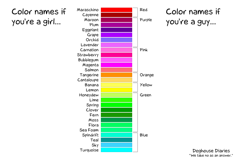
The old trope is that males are less sensitive to colour distinctions:^[Though see https://blog.xkcd.com/2010/05/03/color-survey-results/ for a more nuanced take.]
Seeing what others see {#seeing-what-others-see}
About one man in twelve, and one woman in two hundred,
sees colour differently from the palette designer.
The most common form, deuteranopia, confuses reds with greens —
which is precisely the pairing a "stop/go" palette relies on.
{autograph} gives you two functions for checking this.
simulate_colorblind() shows you a set of colours as such a viewer sees them,
and check_separation() scores how far apart colours are,
taking the worst case across normal vision and each type of colour blindness.
A score below 10 means two colours are easily confused,
10 to 25 that they are separable but close,
and above 25 that they are comfortably distinct.
# A red and a green that look quite different to most viewers
check_separation(c("#B7352D", "#627313"))
# But not to everyone
simulate_colorblind(c("#B7352D", "#627313"), "deutan")
Run the code, then try "protan" or "tritan" instead of "deutan".
How far the simulation goes is set by severity.
Full severity, the default, is dichromacy:
deuteranopia, protanopia, tritanopia.
A lower severity is anomalous trichromacy —
deuteranomaly, protanomaly — which is the more common condition,
and which the paragraph above named without being able to show you.
simulate_colorblind(c("#B7352D", "#627313"), "deutan", severity = 1)
simulate_colorblind(c("#B7352D", "#627313"), "deutan", severity = 0.4)
You can also look at a whole graph the way another viewer would,
by mapping the simulated colours back onto it.
graphr(fict_lotr, node_colour = "Race")
graphr(fict_lotr, node_colour = "Race") +
  ggplot2::scale_fill_manual(values = simulate_colorblind(ag_qualitative(6), "deutan"))
Much of this work is already done for you.
Each theme's palette is reordered when the theme is set,
so that the colours a graph uses first are the ones that stay distinct
for every viewer,
and each divergent palette pairs a warm pole with a cool one
rather than a red with a green.
stocnet_theme("iheid")
round(check_separation(ag_qualitative(4)))
# The closest pair among those four colours
min(check_separation(ag_qualitative(4)), na.rm = TRUE)
stocnet_theme("default")
::: {.callout}
Going further:
The "rainbow" theme is the exception, and is left in the order of the
spectrum, since that fidelity is its point.
A spectrum is not a colour-blind safe scheme:
its reds and greens are the pair that red-green colour blindness cannot
separate.
Choose it where the order of your categories is itself meaningful,
and check the result with check_separation().
Where you need particular colours in an institutional palette,
match_color() finds the closest the palette has to those you ask for.
:::
Greyscale {#greyscale}
Other times colour may not be desired.
Some publications require greyscale images,
and a figure may be photocopied whether or not you meant it to be.
A greyscale device keeps the luminance of a colour and throws the rest away,
so two colours of the same lightness merge, however different their hues.
This is why ColorBrewer marks a palette print-safe and photocopy-safe
separately from marking it colour-blind safe:
they are different questions, and a palette can pass one and fail the other.
simulate_colorblind() answers the second with type = "grey",
and check_separation() reports the greyscale distances beside its own score.
check_separation(ag_qualitative(4))
The matrix is what every viewer can see.
The line beneath it is what survives a photocopier.
Most institutional palettes separate their categories by hue,
so most of them collapse in greyscale.
To draw in greyscale from the start,
replace _hue from above with _grey (note the 'e' spelling):
graphr(fict_lotr,
           node_colour = "Race") +
  ggplot2::scale_fill_grey()
As you can see, greyscale is more effective for continuous variables
or for very few discrete categories than for the six categories used here.
If you need to distinguish several categories in print,
consider combining greyscale with node_shape,
or use the "bw" theme, which is designed for this purpose.
stocnet_medium("print") is the companion to this;
see Where will it be seen? below.
Manual override {#manual-override}
Or we may want to choose particular colours for each category.
This is pretty straightforward to do with ggplot2::scale_fill_manual().
Some common colour names are available,
but otherwise hex colour codes can be used for more specific colours.
Unspecified categories are coloured (dark) grey.
graphr(fict_lotr,
           node_colour = "Race") +
  ggplot2::scale_fill_manual(
    values = c("Dwarf" = "red",
               "Hobbit" = "orange",
               "Maiar" = "#DEC20B",
               "Human" = "lightblue",
               "Elf" = "lightgreen",
               "Ent" = "darkgreen")) +
  labs(fill = "Colour")
Where will it be seen? {#where-will-it-be-seen}
A theme says how a plot should look.
Where it will be seen is a separate question,
and the answer changes more often than the theme does.
The same institutional theme has to serve a figure worked on at a desk,
projected in a lecture theatre, printed in an article,
and read on a phone in a narrow column.
Each of those wants a different size of text,
and one of them wants a different background.
stocnet_medium() sets this, and leaves the theme alone.
stocnet_medium()
stocnet_medium("presentation")
graphr(fict_lotr, node_colour = "Race")
stocnet_medium("screen")
The media are "screen" (the default), "presentation", "mobile",
and "print".
The first three differ in the size of their text;
ag_size() reports the multiplier in force.
"print" leaves the text alone and draws on white,
whatever ground the theme prefers,
since a dark or tinted ground costs ink and is often not reproduced.
As with stocnet_theme(), persist = TRUE remembers your choice.
The medium scales text, not marks.
A node's size is relative to the layout it sits in,
so enlarging the nodes without enlarging the layout would only crowd it.
Use node_size in graphr() where a figure needs larger nodes too.
Nor does the medium set the size of the file you write.
Give ggsave() the width, height, and resolution to match;
see Exporting plots below.
::: {.callout}
Going further:
A small figure limits how much it can carry, not just how large the type is.
Keep a legend to about seven keys, and graphs() to about three panels.
graphr() says so when a colour or shape legend grows past that,
because past it a reader stops matching keys to marks and starts guessing.
Splitting one crowded figure into two that each make a single point
is almost always better than shrinking the type until it fits.
:::
::: {.callout}
In brief: stocnet_theme() sets a theme once for all subsequent
graphs and plots, with institutional and stylistic palettes included,
and persist = TRUE keeps it for future sessions.
Individual graphs can still be adjusted by appending
ggplot2::scale_fill_*() functions —
_hue() for a different palette, _grey() for print,
_manual() for hand-picked colours —
and simulate_colorblind(), check_separation() and check_contrast() check
that your palette works for colour-blind viewers, in greyscale, and as text.
stocnet_medium() then sizes the result for where it will be seen.
:::
Layouts
On this page:
Spectral ·
Layered ·
Circular ·
Grid ·
Force-directed ·
Manual
Unlike the maps and scatterplots you may be used to,
where a node is drawn on a network graph is usually not data.
Its position is chosen by an algorithm to make the structure readable,
and a different algorithm would have put it somewhere else.
Knowing which algorithm drew a graph — and so what can and cannot be read off
the positions in it — is the point of this section.
It helps to sort layouts by how much of a node's position is data.
We start with layouts where both coordinates mean something,
and work our way down to those where the position
is only there to keep the picture legible:
| Layouts | What a node's position means |
|---|---|
| Spectral: "eigen", "scaling", "correspondence" | Both axes are calculated from the network |
| Layered: "layered", "railway", "lineage", "ladder" | One axis is data: a mode, a rank, a generation, a year |
| Circular: "concentric", "circle" | The ring a node is on, or its place around it, can be data |
| Grid: "grid", or any layout with layout_snap = TRUE | Regular positions, chosen to keep labels apart |
| Force-directed: "stress", "fr", "kk" | A compromise, chosen to keep the whole drawing legible |
| Manual: x = and y = | Whatever you decide |
Here is one network drawn by one layout from each of the first five rows.
Nothing about the network changes from panel to panel; only what you can read from it does.
sw_panel <- function(p, title) {
  p + ggtitle(title) + labs(caption = NULL) +
    theme(legend.position = "none", plot.title = element_text(size = 10))
}
patchwork::wrap_plots(list(
  sw_panel(graphr(ison_southern_women, layout = "scaling", labels = FALSE),
           "Spectral: both axes are data"),
  sw_panel(graphr(ison_southern_women, layout = "layered", labels = FALSE),
           "Layered: one axis is data"),
  sw_panel(graphr(ison_southern_women, layout = "concentric", labels = FALSE),
           "Circular: the ring is data"),
  sw_panel(graphr(ison_southern_women, layout = "grid", labels = FALSE),
           "Grid: regular positions"),
  sw_panel(graphr(ison_southern_women, layout = "stress", labels = FALSE),
           "Force-directed: legible positions")
), nrow = 2)
Graph layouts available in the {igraph}, {ggraph}, {graphlayouts},
and {autograph} packages can be used in graphr().
These can be specified using the layout argument.
For these examples we will mostly use ison_southern_women,
a classical r gloss("two-mode","twomode") network of women attending events,
because two-mode networks make the differences between layouts
especially visible.
Spectral layouts {#spectral-layouts}
Spectral layouts are the nearest a network graph comes to a scatterplot.
Both axes are calculated from the network,
and a node's coordinates are its scores on them,
so that nodes drawn together are similar in some measured sense.
{autograph} offers three, which differ in what they take 'similar' to mean:
- the eigenvector layout draws together nodes that are tied to the same others;
- multidimensional scaling draws together nodes that are few steps apart;
- correspondence analysis draws together nodes whose rows in a table of ties look alike.
All three are careful about position and careless about legibility:
nodes pile up on top of each other, and ties run long and cross often.
The rest of this page gradually reverses that trade.
Eigenvector layout {#eigenvector}
The eigenvector layout starts from a matrix.
The Laplacian of a network is a table with a row and a column for every node,
which records each node's degree on its diagonal
and marks each pair of nodes that are tied.
Like any such table, it can be broken down into eigenvectors:
a series of axes, each of which gives every node a single score.
The "eigen" layout takes two of them, the two along which the scores
change least from a node to the nodes it is tied to, and draws one as x and the other as y.
Three things follow from choosing axes this way.
Tied nodes get similar scores, so a tightly knit group is drawn close together.
Nodes tied to exactly the same others get exactly the same scores,
and are drawn on top of each other.
And the few nodes that connect one group to another
are pulled out along an axis, somewhere between the two.
You can see all three in about the simplest network that has groups at all:
three groups of four, in which everyone is tied to everyone else in their group,
joined in a chain by two ties.
three_groups <- add_ties(create_components(12, membership = rep(1:3, each = 4)),
                         c(4, 5, 8, 9))
(graphr(three_groups, layout = "eigen", node_size = 5) +
    ggtitle("Eigenvector layout") |
    graphr(three_groups, layout = "stress", node_size = 5) +
    ggtitle("Default layout, for comparison"))
Both panels draw the same twelve nodes, but on the left you can count only seven.
In each of the groups at the ends of the chain,
three members share all their ties, and so share one position;
the member that holds the tie to the middle group is drawn a little towards it.
The middle group, tied to both of the others, is drawn between them.
The drawing has lost almost everything about the network
except the one thing it is for: there are three groups here,
this is the order they come in, and these are the nodes that join them.
So this is how to read an eigenvector layout:
- do read which cluster a node falls in, and which side of an axis it is on:
the first axis marks the deepest division in the network;
- do read the nodes strung out between clusters as the ones that connect them;
- do not read a distance as a number of steps, or count the nodes in a clump,
since several may be hiding behind one.
Now draw the Southern Women this way.
Which women are drawn on the same side as which events?
graphr(ison_southern_women, layout = "eigen") + ggtitle("Eigenvector")
Real networks are rarely as tidy as three groups in a chain,
but the same reading applies:
the women and events at either end of the horizontal axis
are those that had least to do with each other,
and those drawn between them took part on both sides.
Multidimensional scaling {#scaling}
Of similar purpose are multidimensional scaling (MDS) techniques,
which visualise the similarity between nodes in terms of their proximity
in a two-dimensional (or more) space.
The "scaling" layout places the nodes so that the distance drawn between them
stands for the number of steps between them in the network.
graphr(ison_southern_women, layout = "scaling") + ggtitle("Multidimensional Scaling")
Note that this layout is drawn with the axes labelled,
whereas you may have noticed that the other graphs are not.
That is because here the coordinates can be read:
two nodes drawn twice as far apart are, more or less, twice as far apart.
The axes are drawn on one scale for the same reason.
The layout scales the whole network where it is small enough for that,
using "mds" from {igraph},
and otherwise approximates the scaling from a sample of the nodes
using "pmds" (or pivot MDS) from {graphlayouts}.
You can still call each of these directly, but since they are both used in "scaling",
dispatch can be automatic, based on the size and structure of the network.
"More or less" is doing some work in that sentence.
A network usually has more structure than two dimensions alone can hold,
so some of the distances drawn will not match the distances in the network.
How far they miss is called the stress of the drawing,
and the caption under the plot reports it, as a percentage, where zero would be a perfect drawing.
The next page, Checking layouts, shows how to read that number,
and how to obtain it for any other layout.
question("Can we interpret the distance between nodes in spectral and MDS layouts?",
  answer("Yes",
         correct = TRUE,
         message = "That's right — in these layouts proximity reflects measured (dis)similarity, though how far to trust it is another question. The stress score reported under a \"scaling\" layout is what answers that one."),
  answer("No",
         message = "Unlike force-directed layouts, spectral and MDS layouts place nodes according to calculated similarities, so distances do carry meaning here."),
  allow_retry = TRUE
)
Correspondence analysis {#correspondence}
Whereas scaling lays out nodes by their distances from each other,
correspondence analysis (CA) lays them out by the similarity of their ties.
This is useful where nodes may not be tied to each other at all,
but can be tied to the same others, such as in a two-mode network.
Correspondence analysis takes a rectangular table ---
here the incidence matrix of the Southern Women dataset,
one row for each woman and one column for each event ---
and places its rows and its columns in one space.
graphr(ison_southern_women, layout = "correspondence") + ggtitle("Correspondence Analysis")
We can see the similarity to the eigenvector layout above,
but here the axes are labelled with the share of the network's r gloss("inertia") they hold.
Inertia is the CA analogue of variance in PCA.
It measures the total dispersion of points (rows and columns) in the cloud around the centroid,
computed as the chi-square statistic of the table divided by the total sample size (N).
In other words, inertia tell us how far the ties depart from what one would expect
if every woman attended events in the same proportion as every other.
A network whose nodes all had much the same ties would have almost none.
Since the two dimensions hold different shares here,
we can see where to put the emphasis of our interpretation.
Because the first dimension holds twice as much as the second,
what distinguishes nodes most runs along the x-axis rather than the y-axis.
Whether those shares are large enough for the plot to be worth interpreting
is a question for the next page, Checking layouts.
One thing to keep in mind whenever you read a correspondence analysis:
while the distances among nodes of the same mode are interpretable,
distances between nodes from different modes are not necessarily interpretable.
That is, a woman drawn near an event is not necessarily an attendee of it.
Only the distances within a mode can be read this way:
two women drawn together attended similar events,
and two events drawn together were attended by similar women.
These plots are often misread this way.
For a directed network, each node has two profiles:
who it sends ties to, and who it receives them from.
By default the layout reads a tie in either direction,
so that each node has one position;
direction = "out" and direction = "in" read one profile or the other.
For a signed network there is no correspondence analysis at all,
since the method divides by the mass of each node
and a negative tie has no such reading.
double = TRUE splits each tie into a positive and a negative part,
so that a node is placed by both who it likes and who it dislikes.
question("In a `\"correspondence\"` layout of `ison_southern_women`, Helen is drawn closer to event E9 than to any other event. What does that tell us?",
  answer("Less than it appears: only distances within a mode can be read",
         correct = TRUE,
         message = "That's right — a row point near a column point is not a claim about the two of them. Helen did not attend E9 at all. Compare women with women, and events with events."),
  answer("That Helen attended E9",
         message = "Not necessarily. The two modes share a pair of axes, but the distance between a woman and an event is not a distance you can read. Compare women with women instead."),
  answer("That Helen was the only woman not to attend E9",
         message = "The plot says nothing of the kind. A distance between the two modes carries no reading at all; only distances within a mode do."),
  allow_retry = TRUE
)
Layered layouts {#layered-layouts}
Layered layouts give up one of the two axes.
One axis is still data — it says which layer a node belongs to —
while the other is used only to arrange the nodes within each layer so that
their ties cross as little as possible.
These layouts are best suited for directed acyclic graphs, two-mode networks,
or other data with a natural ordering.
{autograph} offers four, and they are one layout drawn four ways.
Two things vary: which axis the layers run along, and whether the nodes
line up across them. The names say which is which — a railway lies flat,
a ladder stands up:
| | Layers stacked flat | Layers standing up |
|--------------------------|---------------------|--------------------|
| Nodes spaced by their ties | "layered" | "lineage" |
| Nodes lined up across layers | "railway" | "ladder" |
graphr(ison_southern_women, layout = "bipartite") + ggtitle("Bipartite")
graphr(ison_southern_women, layout = "layered") + ggtitle("Layered")
graphr(ison_southern_women, layout = "railway") + ggtitle("Railway")
Note that "layered" and "railway" use a different algorithm to
{igraph}'s "bipartite", and generally perform better,
especially where there are multiple layers.
Whereas "layered" tries to position nodes to minimise overlaps,
"railway" sequences the nodes in each layer to a grid
so that nodes are matched as far as possible.
For the "layered" layout you can also steer which set sits where by
passing a center argument — "events" or "actors" for a two-mode
network, or the name of a particular node — which helps when the default
places the less interesting set on top.
graphr(ison_southern_women, layout = "layered", center = "events")
If you want to flip the horizontal and vertical,
you could flip the coordinates, or use "lineage",
which is the same layout with the axes exchanged.
graphr(ison_southern_women, layout = "lineage") + ggtitle("Lineage")
These layouts serve both multimodal and directed acyclic networks.
A genealogical network offers the clearest case:
every tie points from an earlier generation to a later one.
Where a force-directed layout obscures this ordering,
graphr() uses the "layered" layout to make it clear.
Draw the parent ties among the characters of Westeros.
thrones <- to_layer(fict_thrones, "parent")
graphr(thrones)
This layout tries to minimise two costs.
The first is which layer each node goes in. Ranking each node
by its distance from a root sounds right — a row is then a generation — but it
pins a parent whose only child is born several generations later to the top
row, and manufactures a long tie to reach them.
The ranks argument chooses the rule,
and check_span() reports how many rows each tie crosses,
so you can measure the difference.
thrones <- to_layer(fict_thrones, "parent")
spans <- sapply(c("generation", "compact", "tight"), function(r) {
  span <- check_span(graphr(thrones, ranks = r))
  c(total = attr(span, "total"), `over one row` = mean(span > 1), max = max(span))
})
round(t(spans), 3)
"generation" is the distance-from-a-root rule and
"compact" is the one {igraph} uses in its Sugiyama layout.
"tight", the default, minimises total tie length while
still pointing every tie down at least one row.
Note that the longest tie is the same under all three.
The second cost is where each node sits within its row.
check_offset() reports how far each tie travels sideways,
as a share of the width of the drawing,
so a tie that drops straight down scores zero.
Again, you are wanting to minimise this,
and the alignment argument chooses the rule.
Compare the two alignments.
thrones <- to_layer(fict_thrones, "parent")
c(straight = attr(check_offset(graphr(thrones)), "mean"),
  rungs = attr(check_offset(graphr(thrones, alignment = "rungs")), "mean"))
alignment = "rungs" gives every row the same spacing,
which is what "railway" and "ladder" are for.
The default, "straight", pulls each node towards its parents and children instead,
which is what makes the families read as families.
ranks also accepts a node attribute, instead of one of those three rules.
Then the layers are that attribute's values, and nodes are placed along the
axis in proportion to them rather than at even steps,
so a network of dated nodes is drawn as a timeline.
Rank the adolescents by a year of your choosing.
ison_adolescents |> as_stocnet() |>
  mutate_nodes(year = rep(c(1985, 1990, 1995, 2000), times = 2),
               label = paste0(label, " (", year, ")")) |>
  graphr(layout = "lineage", ranks = "year")
Other layered layouts include:
- Tree:
"tree"
- Dominance layouts
Circular layouts {#circular-layouts}
Circular layouts give up Cartesian axes altogether and
arrange nodes around (potentially concentric) circles,
such that crossings are minimised and adjacent nodes are located close together.
What is left that can be data is the ring a node is on:
in some cases, the ring can be specified by attribute or mode.
graphr(ison_southern_women, layout = "concentric") + ggtitle("Concentric")
The "concentric" layout can also place nodes on rings by a grouping you
choose: pass a membership argument (a node attribute name, or a vector the
same length as the number of nodes). Ring the Lord of the Rings characters
by their race.
graphr(fict_lotr, layout = "concentric", membership = "Race")
Other such layouts include:
- circular:
"circle"
- sphere:
"sphere"
- star:
"star"
- arc or linear layouts:
"linear"
Grid layouts {#grid-layouts}
Grid layouts arrange nodes at regular Cartesian coordinates.
Here the positions are no longer data at all:
they are evenly spaced because even spacing is tidy.
These can be useful for making sure all nodes' labels are visible,
but horizontal and vertical lines can overlap,
making it difficult to distinguish whether some nodes are tied or not.
graphr(ison_southern_women, layout = "grid") + ggtitle("Grid")
Other grid layouts include:
- orthogonal layouts for e.g. printed circuit boards
- grid snapping for other layouts
That last point deserves a demonstration. Rather than committing to a full
grid, graphr()'s layout_snap = TRUE argument keeps whatever layout you asked for
but snaps its coordinates onto a grid — trading a little positional accuracy
for the label legibility of a grid. Compare the stress layout with its
snapped version.
(graphr(fict_lotr) + ggtitle("stress") |
   graphr(fict_lotr, layout_snap = TRUE) + ggtitle("stress + snap"))
question("What does layout_snap = TRUE do to the layout you asked for?",
  answer("It keeps that layout, but moves each node onto the nearest grid coordinate",
         correct = TRUE,
         message = "Exactly — the arrangement stays recognisable, and the nodes just shuffle onto tidier positions. <img src='https://media1.tenor.com/m/06gR6YNAA6IAAAAd/family-guy-cartermiroquai.gif' alt='gif of a cartoon character energetically rearranging the living room furniture'/>"),
  answer("It replaces that layout with the grid layout",
         message = "That is layout = 'grid'. With layout_snap = TRUE the chosen layout is computed first, and only then rounded onto a grid."),
  answer("It fixes the layout so that it is the same each time it is run",
         message = "Some layouts, such as 'stress', are already deterministic. Snapping is about grid coordinates, not repeatability."),
  answer("It removes overlapping labels",
         message = "Snapping often helps label legibility, but it moves nodes rather than labels. Use label_repel and label_dist for labels."),
  random_answer_order = TRUE,
  allow_retry = TRUE
)
Force-directed layouts {#force-directed-layouts}
Force-directed layouts complete the trade this page has been making.
They give up position as data entirely,
in exchange for a drawing in which tied nodes sit near each other,
untied nodes keep apart, and the ties are of a similar and readable length.
This is why one of them is the default layout for most networks,
and why you have been looking at them since your first graph.
Force-directed layouts update some initial placement of vertices
through the operation of some system of metaphorically-physical forces.
These might include attractive and repulsive forces.
(graphr(ison_southern_women, layout = "kk") + ggtitle("Kamada-Kawai") |
   graphr(ison_southern_women, layout = "fr") + ggtitle("Fruchterman-Reingold") |
   graphr(ison_southern_women, layout = "stress") + ggtitle("Stress Minimisation"))
The Kamada-Kawai (KK) method inserts a spring between all pairs of vertices
that is the length of the graph distance between them.
This means that edges with a large weight will be longer.
KK offers a good layout for r gloss("lattice","lattice")-like networks,
because it will try to space the network out evenly.
The Fruchterman-Reingold (FR) method uses an attractive force between
directly connected vertices,
and a repulsive force between all vertex pairs.
The attractive force is proportional to the edge's weight,
thus edges with a large weight will be shorter.
FR offers a good baseline for most types of networks.
The Stress Minimisation (stress) method is related to the KK algorithm,
but offers better runtime, quality, and stability and so is generally preferred.
Indeed, {autograph} uses it as the default for most networks.
It has the advantage of returning the same layout each time it is run
on the same network.
question("Can we interpret the distance between two nodes in a force-directed layout as a precise measure of how closely they are related?",
  answer("No",
         correct = TRUE,
         message = "That's right — force-directed layouts are illustrative. Nearby nodes are often closely connected, but distances are a by-product of the algorithm, not a measurement to cite. The force moves the nodes, but it does not measure them. <img src='https://giffiles.alphacoders.com/131/13131.gif' alt='gif of yoda moving things with the force'/>"),
  answer("Yes",
         message = "Careful — two nodes can end up near each other simply because the algorithm ran out of better places to put them. Use spectral or MDS layouts if you need interpretable distances. No mistakes here though, just a happy little accident. <img src='https://media1.tenor.com/m/XP2eqZczZ2MAAAAC/bob-ross-happy.gif' alt='gif of Bob Ross smiling in front of a painting'/>"),
  allow_retry = TRUE
)
Other force-directed layouts available include:
- Simulated annealing (Davidson and Harel 1993):
"dh"
- Graph embedder (Frick et al. 1995):
"gem"
- Graphopt (Schmuhl):
"graphopt"
- Distributed recursive graph layout (Martin et al. 2008):
"drl"
Manual layouts {#manual-layouts}
Whatever their differences, all these layout algorithms do the same job:
they return a table of node coordinates.
Nothing stops you computing that table yourself,
inspecting it, adjusting a coordinate or two,
and handing the result back to graphr() via its x and y arguments.
This is handy when a layout is almost right —
say one label sits awkwardly, or you want a particular node set apart —
or when you need the same hand-tuned positions across several figures.
Compute a stress layout for fict_lotr, inspect the coordinate table,
banish Gollum to the top-right corner, and re-graph.
lo <- ggraph::create_layout(as_tidygraph(fict_lotr), layout = "stress")
head(lo[, c("name", "x", "y")])
lo$x[lo$name == "Gollum"] <- max(lo$x) + 1
lo$y[lo$name == "Gollum"] <- max(lo$y) + 1
graphr(fict_lotr, x = lo$x, y = lo$y)
The same trick lets you reuse a layout across plots
(compute once, pass the same x/y to each call),
which keeps node positions identical between figures —
useful when readers need to compare them.
::: {.callout}
Going further:
{autograph} also provides its own special-purpose layouts —
"configuration", "correspondence", "levels", "matching",
"scaling", "valence",
and the layered family —
documented at ?layout_layered and friends.
Several layouts take a layout-specific extra argument (passed through ...)
to control how nodes are ordered: "concentric" a membership,
"levels" a level, and the layered layouts ranks — each a node attribute
name or a vector. See ?graphr for the full list.
:::
::: {.callout}
In brief: Pass layout = to graphr() to choose among
spectral ("eigen", "scaling", "correspondence"),
layered ("layered", "railway", "lineage"),
circular ("concentric", "circle"),
grid, and force-directed ("stress", "fr", "kk") layouts.
The order matters: spectral layouts place nodes by measured similarity,
so their positions can be read;
layered layouts make one axis mean something, which suits two-mode or hierarchical data;
force-directed layouts are illustrative — do not over-interpret distances in them.
And since every layout is just a table of coordinates,
you can always compute one with ggraph::create_layout(),
adjust it, and pass it back via graphr()'s x and y arguments.
:::
Checking layouts
On this page:
Legibility ·
Layers ·
Faithfulness ·
Free play
The last page sorted layouts by what their positions mean.
This page asks a second question of any one drawing: is it any good?
There are two quite different ways for a drawing to be good.
It can be legible: easy on the eye, with ties you can follow.
And it can be faithful: its distances can stand for distances in the network.
Each check_*() function below scores one of these qualities,
and each scores a drawing rather than the network it draws,
so that two layouts of the same network can be compared.
Legibility {#check-legibility}
Researchers who study graph drawing have identified a number of features
that make a drawing easier or harder to read.
Each of the following four comes with a pair of drawings of one small network:
the same nodes and the same ties, only placed differently.
The score in each title is calculated from the drawing beneath it.
Crossings {#check-crossings}
Ties that cross are hard to follow, and a reader can mistake a crossing for a node.
check_crossings() counts the crossings in a drawing.
A ring of eight nodes can be drawn with none at all;
place the same nodes around the same circle in another order,
and the same eight ties cross repeatedly.
(A graph that can be drawn with no crossings is called
planar; many cannot.)
title_score <- function(p, label, value) p + ggtitle(paste0(label, ": ", value))
on_circle <- function(n, order = seq_len(n)) {
  angle <- 2 * pi * (order - 1) / n
  list(x = cos(angle), y = sin(angle))
}
ring <- create_ring(8)
set.seed(3)
tidy <- on_circle(8)
mixed <- on_circle(8, sample(8))
p1 <- graphr(ring, x = tidy$x, y = tidy$y, node_size = 5)
p2 <- graphr(ring, x = mixed$x, y = mixed$y, node_size = 5)
(title_score(p1, "Crossings", attr(check_crossings(p1), "total")) |
    title_score(p2, "Crossings", attr(check_crossings(p2), "total")))
Slopes {#check-slopes}
A drawing whose ties run in only a few directions looks ordered,
and one whose ties run in every direction looks busy.
check_slopes() counts the different slopes that the ties are drawn at.
A r gloss("lattice") drawn on a grid needs only three;
the same lattice drawn around a circle needs many more.
lattice <- create_lattice(9)
p1 <- graphr(lattice, layout = "grid", node_size = 5)
p2 <- graphr(lattice, layout = "circle", node_size = 5)
(title_score(p1, "Slopes", attr(check_slopes(p1), "distinct")) |
    title_score(p2, "Slopes", attr(check_slopes(p2), "distinct")))
Lengths {#check-lengths}
Long ties are hard to follow from one end to the other,
and ties of very different lengths suggest differences that are not in the data:
a long tie reads as a weak or distant one, whether or not it is.
check_lengths() measures each tie as a share of the diagonal of the drawing,
and reports their total, their maximum, and how much they vary
("cv", the coefficient of variation, which is zero where every tie is the same length).
Pull one node of the ring away from the others,
and two ties stretch while the rest stay as they were.
ring <- create_ring(8)
tidy <- on_circle(8)
pulled <- tidy
pulled$x[5] <- pulled$x[5] * 3
p1 <- graphr(ring, x = tidy$x, y = tidy$y, node_size = 5)
p2 <- graphr(ring, x = pulled$x, y = pulled$y, node_size = 5)
(title_score(p1, "Variation in length", round(attr(check_lengths(p1), "cv"), 2)) |
    title_score(p2, "Variation in length", round(attr(check_lengths(p2), "cv"), 2)))
Angles {#check-angles}
Where several ties meet at a node, they are easiest to tell apart when they
leave it in well separated directions.
check_angles() reports the smallest angle between two ties at each node,
and the smallest of those is the angular resolution of the drawing.
A star with six leaves can give every tie 60° of room;
gather the same leaves on one side of the centre, and the ties crowd together.
star <- create_star(7)
around <- on_circle(6)
fan <- seq(-40, 40, length.out = 6) * pi / 180
p1 <- graphr(star, x = c(0, around$x), y = c(0, around$y), node_size = 5)
p2 <- graphr(star, x = c(0, cos(fan)), y = c(0, sin(fan)), node_size = 5)
(title_score(p1, "Smallest angle", paste0(round(attr(check_angles(p1), "min")), "°")) |
    title_score(p2, "Smallest angle", paste0(round(attr(check_angles(p2), "min")), "°")))
All at once {#check-drawing}
check_drawing() runs all four of these checks at once, beside check_stress(),
which we will come to under Faithfulness below.
Compare a stress layout with a circle.
sw_stress <- graphr(ison_southern_women, layout = "stress")
sw_circle <- graphr(ison_southern_women, layout = "circle")
rbind(stress = check_drawing(sw_stress), circle = check_drawing(sw_circle))
Every column is read downwards except angle_min, which is read upwards.
Fewer crossings, fewer slopes, shorter ties, more even ties, and a wider
smallest angle all make a drawing easier to read.
nodes, ties and angle_ideal are context rather than scores.
angle_ideal is the widest smallest angle the degrees of this network allow,
so angle_min is read as a share of it.
The floors are worth knowing as well:
a network of this many ties cannot be drawn without crossings at all,
and no drawing of it can use fewer slopes than half its largest degree.
No layout wins on every measure.
The circle draws every node on one ring, which costs it crossings and length:
it draws many times the crossings of the stress layout, and three times the
total tie length. It buys the other measures with the same ring:
fewer slopes, ties of a more even length, and more room between the ties that
meet at a node. Its stress is the worse of the two,
because a layout that never set out to draw the path distances
scores poorly on them by design.
A few other qualities are sometimes asked of a drawing but are not measured here:
the number of bends in its ties
(which graphr()'s edge_bundle argument sets, rather than the layout),
the size and aspect ratio of the box it fits in,
and how well it displays the symmetries of the network.
Layers {#check-layers}
Layered layouts have two legibility checks of their own,
which you met with the family tree of Westeros in Layered layouts:
check_span() counts how many rows each tie crosses,
and check_offset() measures how far each tie travels sideways.
Both are costs. A tie that runs to the next row is easy to follow;
one that passes over a row has to find its way between the nodes on it.
Each of the six ties in a small tree runs to the next row.
Move one leaf down a row, and its tie crosses two rows instead of one,
so that the total over all the ties rises from six rows to seven.
tree <- create_tree(7, directed = TRUE)
p1 <- graphr(tree, layout = "layered", node_size = 5)
lowered <- p1$data$y
lowered[4] <- min(lowered) - 0.5
p2 <- graphr(tree, x = p1$data$x, y = lowered, node_size = 5)
(title_score(p1, "Longest tie, in rows", max(check_span(p1))) |
    title_score(p2, "Longest tie, in rows", max(check_span(p2))))
Faithfulness {#check-faithfulness}
A legible drawing is not necessarily a faithful one.
Where a layout claims that its distances are data,
as the spectral layouts on the last page did, we should ask how far to believe it.
Stress {#check-stress}
Stress measures the disagreement between the distances drawn
and the distances in the network, counted as the number of steps from one node to another.
It is a percentage of the network distances,
such that zero would represent a perfect drawing.
A path of seven nodes drawn as a straight line is one:
every pair of nodes is drawn exactly as far apart as it is steps apart.
Bend the same path around a circle,
and its two ends, six steps apart, are drawn almost as neighbours.
path <- delete_ties(create_ring(7), 7)
bent <- on_circle(8)
p1 <- graphr(path, x = 1:7, y = rep(0, 7), node_size = 5)
p2 <- graphr(path, x = bent$x[1:7], y = bent$y[1:7], node_size = 5)
(title_score(p1, "Stress", paste0(round(100 * check_stress(p1)), "%")) |
    title_score(p2, "Stress", paste0(round(100 * check_stress(p2)), "%")))
How low is low? Kruskal (1964),
who introduced the score, recommends 20% as poor, 10% as fair, 5% as good,
and 2.5% as excellent.
Those figures were established for psychometric data though.
Networks typically contain a lot more structure,
which is hard to capture in just two dimensions,
so a 20% threshold is often too demanding.
For networks, a score near 30% is quite common,
and means the clustering can be interpreted though perhaps the distances should not be interpreted as exact.
Above 40% and the plot does not really show any interpretable structure;
graphr() will alert you in the console where the score is above 30%.
By contrast, a stress score near 5% is rare and worth trusting.
Note that this stress score is not only for the "scaling" layout.
check_stress() measures any drawing the same way,
so layouts can be compared on the same network
(Brandes and Pich 2007):
sapply(c("scaling", "stress", "fr", "circle"),
       function(x) check_stress(graphr(ison_southern_women, layout = x)))
The default "stress" layout scores a little better here,
which is no accident: it minimises a related criterion directly.
What "scaling" adds is the axes and the score,
so that the distances can be read and the reading can be checked.
In addition to stress, the "scaling" layout also reports
how much of the variance in the network's distances the two dimensions drawn hold.
The two numbers answer different questions,
and the comparison above shows how.
Stress belongs to the drawing:
draw this one network four ways and you get four different scores.
The variance explained belongs to the network:
it is the same 31% whichever of the four you draw,
because it asks how much of the structure two dimensions could hold at all.
So read them together.
A low variance explained sets a floor that no layout gets under.
Where two dimensions can hold only a third of the structure,
no arrangement of the nodes will draw the distances faithfully,
and stress tells you how close to that floor this particular drawing gets.
question("A `\"scaling\"` layout reports two numbers: a stress score and a share of the distance variance. One of them would be the same for any other layout of the same network. Which one?",
  answer("The variance explained",
         correct = TRUE,
         message = "That's right — it asks how much of this network's structure two dimensions could hold at all, which no choice of layout changes."),
  answer("The stress",
         message = "Stress scores the drawing rather than the network, so it does change: `check_stress()` reports 31% for `\"scaling\"` and 52% for `\"circle\"` on `ison_southern_women`."),
  answer("Both of them, since both describe the network",
         message = "Only the variance explained describes the network. Stress measures how far one particular drawing gets the distances wrong, so redrawing the network changes it."),
  answer("Neither of them, since both describe the drawing",
         message = "Only stress describes the drawing. The variance explained is read from the network's distances, before any nodes are placed."),
  allow_retry = TRUE
)
Inertia {#check-inertia}
Correspondence analysis has its own measure of how much the two dimensions drawn hold,
which you saw on its axis labels: each one's share of the network's r gloss("inertia").
Each dimension extracted captures a share of this total inertia.
Because it is a share of variance explained,
and not a measure of fit like regression's R-squared,
the scores depend on the number of dimensions.
ison_southern_women has 12 dimensions,
and a total inertia of r round(attr(layout_correspondence(ison_southern_women), "fit")$total, 2).
The top two dimensions (in terms of variance explained) together account for 57% of this total inertia.
Is this good? I.e. is this a presentation of the data that is worth interpreting?
Well, if the inertia were spread evenly across these 12 dimensions,
(any) 2 dimensions would jointly account for about 17% of the variance.
57% is about 3.4 times better than this.
But this flatters because inertia is never spread evenly (Jackson 1993).
The broken stick model offers a more demanding baseline,
asking what two dimensions would hold if the inertia were divided randomly rather than evenly (here 1.3 times better):
bstick <- function(K) sum(sapply(1:2, function(k) mean(1 / (k:K))))
sapply(c("ison_southern_women", "ison_adolescents", "ison_networkers"),
       function(x) {
         fit <- attr(layout_correspondence(get(x)), "fit")
         K <- length(fit$scree)
         c(dimensions = K,
           inertia_drawn = round(sum(fit$inertia), 2),
           vs_even = round(sum(fit$inertia) / (2 / K), 1),
           vs_random = round(sum(fit$inertia) / bstick(K), 1))
       })
ison_adolescents looks the best summarised by two dimensions of three datasets considered at 60%.
However, it is a small network with only seven dimensions to spread across,
so two of them were always going to hold a good deal.
Against the harder baseline it scores below 1,
which is to say two dimensions hold less than dividing the inertia
at random would have given them.
By comparison, ison_networkers looks the worst at 36% and yet summarises best:
it has 31 dimensions, and the top two beat either baseline.
Note that these scores are not verdicts,
but help gauge whether the two dimensions presented are worth interpreting further.
graphr() applies the stricter of the two baselines for you,
noting at the console where two dimensions hold no more inertia
than a random division would have given them.
Cos2 {#check-cos2}
A share of inertia describes the plot as a whole.
But some nodes are better represented by the top two dimensions than others.
A plot can hold most of the network's inertia
and still put one particular node nowhere near where it belongs.
This representation is captured by a measure called r gloss("cos2"):
how much of its position the two dimensions drawn actually hold, from 0 to 1,
where lower is worse.
A node the plane captures badly may be located near the centre of the plot,
not because it is average, but because there is nowhere else to put it.
graphr() names these nodes in the console when it draws the layout,
but you can recover the scores like so:
fit <- attr(layout_correspondence(ison_southern_women), "fit")
round(sort(fit$cos2), 2)
question("Two `\"correspondence\"` plots: one holds 60% of its network's inertia in the two dimensions drawn, the other 36%. Which is the better two-dimensional summary?",
  answer("It depends how many dimensions each network had to begin with",
         correct = TRUE,
         message = "That's right — 60% of seven dimensions is less than dividing the inertia at random would have given, while 36% of thirty-one beats every baseline. Compare each share against its own, not against 100%."),
  answer("The one holding 60%",
         message = "Not necessarily. A share of inertia is measured against however many dimensions the table has. A small network has few, so two of them will hold a good deal whatever its structure."),
  answer("The one holding 36%, since a lower share is harder to achieve",
         message = "Closer, but for the wrong reason — a lower share is not a virtue in itself. What matters is the share compared against what an even spread across the available dimensions would give."),
  answer("Neither, since inertia cannot be compared across networks",
         message = "The raw shares cannot, which is the point. But dividing each by its own even-spread baseline does give you a comparison."),
  allow_retry = TRUE
)
question("Should the inertia percentages a `\"correspondence\"` layout reports be adjusted by the Benzécri correction?",
  answer("No — that correction is for multiple correspondence analysis",
         correct = TRUE,
         message = "That's right. An indicator matrix invents dimensions that deflate every percentage, which is what Benzécri (and Greenacre's adjusted version) put back. A single two-way table invents nothing, so these percentages are already exact."),
  answer("Yes, correspondence analysis always understates its percentages",
         message = "Only multiple correspondence analysis does, and only because of the indicator matrix it is run on. This layout analyses a single two-way table, where the percentages are exact."),
  answer("Yes, but only for two-mode networks",
         message = "The number of modes has nothing to do with it. What would call for a correction is an indicator or Burt matrix, which this layout never builds."),
  allow_retry = TRUE
)
question("A node in a `\"correspondence\"` layout is drawn near the origin. What are the two things that could mean?",
  answer("Its ties are close to average, or the two dimensions hold it badly",
         correct = TRUE,
         message = "That's right — and the cos2 is what tells the two apart. A low cos2 means the node sits somewhere this plane cannot show."),
  answer("It has few ties, or it has many",
         message = "Correspondence analysis divides each node's ties by how many it has, so how many a node has is not what places it. Look at the cos2 instead."),
  answer("Only that its ties are close to average",
         message = "That is one of the two. The other is that the two dimensions drawn hold the node badly, so the origin is simply where it lands. The cos2 separates the cases."),
  allow_retry = TRUE
)
Free play {#checking-free-play}
Your turn: the create_*() functions from {manynet} make networks
with one very regular structure each,
which makes them ideal for finding out what each check rewards.
The code below draws a ring, a star, a lattice, and a tree with one layout,
and checks each drawing.
Change the layout to "stress", "grid", "star", or "tree".
Which network and layout together give the fewest slopes?
The most even ties? The widest smallest angle?
And can you find a layout that draws the lattice without any crossings?
nets <- list(ring = create_ring(12), star = create_star(12),
             lattice = create_lattice(12), tree = create_tree(12))
do.call(rbind, lapply(nets, function(net) {
  check_drawing(graphr(net, layout = "circle"))
}))
::: {.callout}
In brief: A drawing can be checked for how legible it is
and for how faithful it is, and the two often pull apart.
| Check | Function | Better when | A layout that aims for it |
|---|---|---|---|
| Crossings | check_crossings() | lower | "layered", "stress" |
| Slopes | check_slopes() | lower | "grid", "circle" |
| Tie lengths | check_lengths() | shorter and more even | "stress", "fr" |
| Smallest angle | check_angles() | higher | "circle", "star" |
| Rows crossed, sideways travel | check_span(), check_offset() | lower | "layered" and its family |
| Stress | check_stress() | lower | "stress", "scaling" |
| Inertia and cos2 | layout_correspondence() | higher | "correspondence" |
check_drawing() reports the first four and stress together.
No layout wins on every measure, so choose the checks that matter
for what you want your reader to see.
:::
Ew, hairballs
On this page:
Isolates ·
Bundling ·
Backbones
Sometimes no layout helps.
Whichever one you choose, the drawing comes out as a dense hairball,
and check_crossings() only confirms what you can already see.
'Hairball' is a technical term to describe networks with many high-degree nodes and many ties,
where the sheer number of ties obscures any structure that might be in the network.
Autograph includes three arguments that can help with this,
some of which are turned on by default,
so we will need to turn them off to see the effect of each in isolation.
Isolates {#isolates}
First, it is possible that the hairball is not a hairball at all,
but a network with many disconnected components or, especially, r gloss("isolates","isolate"),
that each need to be drawn.
As each r gloss("component") is drawn under a force-directed layout,
the components will repel each other and the r gloss("giant") component will be squeezed into a clump.
The isolates argument in graphr() provides some options for what to do with them instead:
"legend" (the default) drops them from the drawing but records how many there were in the legend,
"caption" notes them in a caption instead,
and "keep" leaves them in place.
Add ten unconnected characters to fict_lotr and compare keeping them with noting them in the legend.
lotr_iso <- to_unlabelled(fict_lotr) |>
  add_nodes(10)
(graphr(lotr_iso, isolates = "keep") + ggtitle("keep") |
   graphr(lotr_iso, isolates = "legend") + ggtitle("legend"))
Bundling ties {#bundling}
The second option is to draw all of the ties 'bundled' together,
which can reveal where the most common paths through the network are.
edge_bundle pulls ties that travel in similar
directions into shared paths — like cabling them together —
so that the main 'highways' of the network stand out.
It is off by default; set edge_bundle = TRUE
(or name a specific algorithm: "force", "path", or "minimal") to switch it on.
ison_lawfirm records 71 lawyers and 2571 ties between them,
which is about as thick a hairball as a network this small can be.
Compare it drawn with and without bundling (turn backbone off too for clearest comparison results).
graphr(ison_lawfirm, backbone = FALSE) + ggtitle("Unbundled") |
  graphr(ison_lawfirm, backbone = FALSE, edge_bundle = "path") + ggtitle("Bundled")
I find this works best with networks that are at least moderately dense,
and sometimes requires a little bit of playing around to get a good result.
Backbones {#backbone}
By contrast, r gloss("backbone") changes which ties the picture is built around.
Ties that carry more weight/structure than expected by a null model local to their endpoints
are in essence what the network would be if it were stripped back to its skeleton.
graphr() then draws the layout according to this skeleton and
fades other ties into the background to further emphasise the main structure.
Most of the time you will not have to ask for this.
Networks of 50+ nodes with 8 ties each on average is drawn this way by default.
But you can specify backbone = FALSE to turns it off, backbone = TRUE to force it on,
or you can name a filter — "disparity", "lans", "noise", "mlf", or "simmelian" — or threshold.
Compare ison_lawfirm drawn with and without its backbone.
(graphr(ison_lawfirm, node_colour = "office", backbone = FALSE) +
   ggtitle("Every tie alike") |
   graphr(ison_lawfirm, node_colour = "office", backbone = TRUE) +
   ggtitle("Backbone"))
The offices are hardly visible on the left. On the right they separate, because
the ties that hold each office together are the ties the filter keeps.
Only the layouts that read tie lengths are laid out this way: "stress" (the
default), "fr", "drl" and "kk". Every other layout, including those whose
coordinates already mean something such as "layered" or "scaling", keeps
its coordinates and only fades its ties. Signed networks have no backbone,
since these null models have no place for a negative weight, and are drawn as
they were.
Bundling and backbones answer the same problem from different ends, so try one
before reaching for both. A bundled tie cannot carry a fading of its own —
bundling merges ties into shared paths — so where both are asked for, the
backbone still shapes the layout but every tie is drawn alike.
For very large real-world networks such as irps_blogs, these work well
together: a backbone picks out the ties that hold the connected core together
(or edge_bundle = TRUE, if you would rather see the paths the ties take than
which of them matter most), while isolates = "legend" keeps its several
hundred unconnected blogs from crowding that core out.
::: {.callout}
In brief: Where a network is too dense or too scattered
for any layout to draw legibly, change what is drawn rather than where:
isolates takes unconnected nodes out of the drawing and into the legend or caption,
edge_bundle gathers ties that run the same way into shared paths,
and backbone lays the network out by the ties that matter most and fades the rest.
:::
Multiple graphs
On this page:
Arrangements ·
Sets ·
Dynamics
Sometimes one graph is not enough:
we want to compare two networks, several subgraphs,
or the same network at different points in time.
Arrangements {#arrangements}
{autograph} uses the {patchwork} package for arranging graphs together,
e.g. side-by-side or above one another.
The syntax is quite straightforward and is used throughout these
vignettes/tutorials.
Basically, you just use + or | to put graphs side-by-side,
and / to put them above one another.
Parentheses can be used to group graphs together.
Try graphing fict_lotr and ison_algebra side-by-side,
and then one above the other.
# Fill in the blanks (this is a template, not runnable code):
# graphr(_____) + graphr(_____)
# graphr(_____) / graphr(_____)
graphr(fict_lotr) + graphr(ison_algebra)
graphr(fict_lotr) / graphr(ison_algebra)
Sets {#sets}
graphr() is not the only graphing function included in {autograph}.
To graph sets of networks together, graphs() makes sure that two
or more networks are plotted together,
using a consistent layout and theme across the panels so that they
can be compared.
This might be a set of ego networks, r gloss("subgraphs","subgraph"),
or waves of a r gloss("longitudinal") network.
graphs(to_subgraphs(fict_lotr, "Race"),
       waves = c(1,2,3,4))
What is happening here is that to_subgraphs() is creating a list of subgraphs
— one per race — and then graphs() is plotting them together at once
with the same set of aesthetic parameters.
The waves argument selects which networks in the list to plot —
here the first four of the six race subgraphs.
Left to its own devices, graphs() plots just the first and last networks
of longer lists, which suits before-and-after comparisons of
longitudinal networks.
When the panels share the same nodes, graphs() computes a single layout and
reuses it across panels so that positions line up and can be compared;
by default it uses the "first" network's layout, but based_on = "last"
or "both" are available. Sharing a layout means every panel has to draw
every node, so in that case isolates are kept in place.
Dynamics {#dynamics}
grapht() is another alternative to graphr(),
this time rendering network changes over time as an animated gif.
Longitudinal networks (with discrete waves)
and dynamic networks (with dated changes) are both supported.
Nodes appear, move, and fade as they enter and exit the network,
and node positions transition smoothly between waves.
Run the following to animate a randomly-evolving version of our
Lord of the Rings network.
(Be patient — rendering an animation takes considerably longer than
drawing a static graph,
and requires the suggested {gganimate} and {gifski} packages.)
fict_lotr |>
  mutate_ties(wave = sample(2001:2012, manynet::net_ties(fict_lotr), replace = TRUE)) |>
  to_waves(cumulative = TRUE) |>
  grapht()
Note that here, as with weight and type in the previous section,
attribute naming matters a little:
a time attribute called wave marks the network as
longitudinal for {manynet},
so to_waves() (and grapht() itself, passed such a network directly)
will split it without being told which attribute to use.
Any other name (say, year) works just as well —
it only needs declaring via to_waves()'s attribute argument.
question("A tie attribute named what marks a network as longitudinal for {manynet}, so that to_waves() and grapht() split it without being told?",
  answer("wave",
         correct = TRUE,
         message = "Yes — name it wave and the waves are found for you, like the pages of a flipbook. Any other name works too, but must be declared via to_waves()'s attribute argument. <img src='https://media1.tenor.com/m/eJEUysVdTxkAAAAd/calvin-and-hobbes-stick-figures-tiger-eating-man-this-was-my-book-stick-figures.gif' alt='gif of a hand flipping through a flipbook of animated stick figures'/>"),
  answer("time",
         message = "Close in spirit, but it is wave that is recognised automatically."),
  answer("year",
         message = "year is a perfectly good name, but you have to declare it via to_waves()'s attribute argument."),
  answer("frame",
         message = "Frames are what the animation renders, not what the network attribute is called."),
  random_answer_order = TRUE,
  allow_retry = TRUE
)
::: {.callout}
Going further:
Animation constrains a few things that a static graph allows.
grapht()'s isolates argument takes "keep" (the default) or "fade"
(fading nodes out in the waves where they have no ties),
rather than graphr()'s "legend"/"caption".
And because they do not translate cleanly from frame to frame,
node_group hulls, edge_bundle, the slight curve on reciprocated ties,
and self-loops are not drawn in animations.
Labels, too, are placed at a fixed offset rather than repelled,
and are hidden by default once a network has more than 30 nodes
(pass labels = TRUE to force them, or select a few as in graphr(),
which is resolved once so the same nodes stay named in every frame).
:::
::: {.callout}
In brief: Combine individual graphs with {patchwork} operators
(+/| beside, / above), graph lists of related networks
with graphs() for comparable panels,
and animate longitudinal or dynamic networks with grapht().
:::
Going further with ggraph
For more flexibility with visualisations,
{autograph} users are encouraged to use the excellent {ggraph} package.
{ggraph} is built upon the venerable {ggplot2} package
and works with tbl_graph and igraph objects.
As with {ggplot2}, {ggraph} users are expected to build
a particular plot from the ground up,
adding explicit layers to visualise the nodes and edges.
This means more typing, but near-total control.
library(ggraph)
ggraph(fict_greys, layout = "fr") +
  geom_edge_link(edge_colour = "dark grey",
                  arrow = arrow(angle = 45,
                                length = unit(2, "mm"),
                                type = "closed"),
                  end_cap = circle(3, "mm")) +
  geom_node_point(size = 2.5, shape = 19, colour = "blue") +
  geom_node_text(aes(label=name), family = "serif", size = 2.5) +
  scale_edge_width(range = c(0.3,1.5)) +
  theme_graph() +
  theme(legend.position = "none")
As we can see in the code above, we can specify various aspects of the plot to
tailor it to our network.
First, we can alter the layout of the network using the layout = argument
to create a clearer visualisation of the ties between nodes.
This is especially important for larger networks, where nodes and ties are more
easily obscured or misrepresented.
In {ggraph}, the default layout is the "stress" layout.
The "stress" layout is a safe choice because it is deterministic and
fits well with almost any graph, but it is also a good idea to explore and try
out other layouts on your data.
More layouts can be found in the {graphlayouts} and {igraph} R packages.
To use a layout from the {igraph} package, enter only the last part of the
layout algorithm name (eg. layout = "mds" for "layout_with_mds").
Second, using geom_node_point() which draws the nodes as geometric shapes
(circles, squares, or triangles), we can specify the presentation of nodes
in the network in terms of their shape (shape=, choose from 1 to 21),
size (size=), or colour (colour=). We can also use aes() to match to
node attributes. To add labels, use geom_node_text() or
geom_node_label() (draws labels within a box). The font (family=),
font size (size=), and colour (colour=) of the labels can be specified.
Third, we can also specify the presentation of edges in the network.
To draw edges, we use geom_edge_link0() or geom_edge_link().
Using the latter function makes it possible to draw a straight line with a
gradient.
The following features can be tailored either globally or matched to specific
edge attributes using aes():
-
colour: edge_colour=
-
width: edge_width=
-
linetype: edge_linetype=
-
opacity: edge_alpha=
For directed graphs, arrows can be drawn using the arrow= argument
and the arrow() function from {ggplot2}.
The angle, length, arrowhead type,
and padding between the arrowhead and the node can also be specified.
For more see David Schoch's excellent resources on this.
question("What is the main trade-off in building a graph directly in {ggraph} rather than with graphr()?",
  answer("You control every layer yourself, but you have to specify each one",
         correct = TRUE,
         message = "Just so — nothing is drawn until you ask for it, so a plain graph takes more typing. Take the restoration into your own hands only when you need that control. <img src='https://media1.tenor.com/m/MFmfCpzr4L0AAAAd/mr-bean-whistlers-mother.gif' alt='gif of Mr Bean taking the restoration of a painting into his own hands'/>"),
  answer("You cannot use {ggplot2} layers with {ggraph}",
         message = "{ggraph} is built on {ggplot2}, so the usual layers, scales, and themes all apply."),
  answer("{ggraph} accepts fewer network classes, so graphr() is always faster to run",
         message = "{ggraph} does expect tbl_graph or igraph objects, but the trade-off here is about control, not speed."),
  answer("Graphs built in {ggraph} cannot be saved with ggsave()",
         message = "They can — both graphr() and ggraph() return ggplot objects, which ggsave() handles alike."),
  random_answer_order = TRUE,
  allow_retry = TRUE
)
::: {.callout}
In brief: Because graphr() returns a ggplot object,
you can go a long way just appending {ggplot2}/{ggraph} layers to it.
When you need full control over every geom,
build the plot directly in {ggraph} —
the skills transfer directly, since {autograph} uses {ggraph} underneath.
:::
Plotting results
While researchers will probably want to start with using graphr()
to visualise the network itself,
{autograph} also offers plot() methods for a number of different
network-related objects,
so that plot(result) "just works" without you needing to remember
a special function for each object.
These include measures of centrality, cohesion, and clustering,
as well as goodness-of-fit plots for network models from packages
such as {RSiena}, {ergm}, and {MoNAn}.
Usefully, all these plots use the same theming system as graphr(),
so that you can set a theme once and have it apply to all your graphs and plots.
Let's try this now,
plotting the distribution of a centrality measure under two themes.
stocnet_theme("default")
plot(node_by_degree(fict_lotr))
stocnet_theme("oxf")
plot(node_by_degree(fict_lotr))
stocnet_theme("default")
Each plot shows the distribution of a node measure across the network —
here how unequal the characters' r gloss("degree") centralities are.
The other measures that can be plotted this way
are introduced in the {netrics} tutorials.
This is a very simple example, but the same principle applies to
all plots in {autograph}:
one can set a theme once and have it apply to all plots,
and one can always add additional {ggplot2} layers
to any plot to further customise it —
titles and labels, but also trend lines, confidence intervals, and so on.
The plot methods for model results are demonstrated in the tutorials
of the packages that produce those results.
Exporting plots
We can save the plots we have made by point-and-click
by selecting 'Save as PDF...' from under the 'Export' dropdown menu
in the plots panel tab of RStudio.
If you want to do this programmatically,
say because you want to record how you have saved it so that you can
e.g. make some changes to the parameters at some point,
this is also not too difficult.
After running the (gg-based) plot you want to save,
use ggsave() to save it to disk:
graphr(fict_lotr, node_colour = "Race")
ggsave("lotr_race.pdf")
ggsave("lotr_race.png", width = 9, height = 6, dpi = 300)
ggsave() infers the file type from the extension
(.pdf, .png, .jpeg, .svg, ...),
saves to your working directory unless you specify a path,
and lets you fix the exact width, height, and resolution (dpi)
your publisher requires.
For print, prefer vector formats (.pdf, .svg),
which stay sharp at any size; see ?ggsave for more.
Animations made with grapht() are saved slightly differently:
use gganimate::anim_save("my_animation.gif"),
which works just like ggsave() but for the last animation rendered.
question("Which file format should you prefer when a publisher asks for a figure that stays sharp at any size?",
  answer(".pdf",
         correct = TRUE,
         message = "Yes — .pdf and .svg are vector formats, so they scale without going blurry. The masterpiece is done: show the world. <img src='https://media1.tenor.com/m/NitBp-Ag5dAAAAAd/alright-the-masterpiece-is-done-show-the-world.gif' alt='gif of a maker declaring that the masterpiece is done and it is time to show the world'/>"),
  answer(".png",
         message = "A .png is a raster format. It is fine for the web, and for print at a high dpi, but it does not scale freely."),
  answer(".jpeg",
         message = "A .jpeg is raster too, and its compression blurs lines and text. Avoid it for graphs."),
  answer(".gif",
         message = "Save a .gif for animations from grapht(), via gganimate::anim_save()."),
  random_answer_order = TRUE,
  allow_retry = TRUE
)
Summary
Well done — you have completed the tutorial on visualising networks!
Along the way, you have learned to use these functions:
| Function | What it does |
|---|---|
| graphr() | graphs any manynet-compatible network with sensible defaults |
| graphr(..., node_colour/node_shape/node_size/node_group) | maps node attributes to aesthetics |
| graphr(..., edge_colour/edge_size) | maps tie attributes to aesthetics |
| graphr(..., edge_arrows) | resizes or removes the arrowheads of directed ties |
| graphr(..., labels, label_repel, label_dist) | chooses which nodes to label, and places the labels |
| graphr(..., layout, snap) | chooses and adjusts the layout algorithm |
| graphr(..., x, y) | places nodes at manually supplied coordinates |
| ggraph::create_layout() | returns a layout's table of node coordinates for tweaking |
| check_drawing(), check_crossings(), check_slopes(), check_lengths(), check_angles() | score how legible a drawing is |
| check_stress() | scores how faithful a drawing's distances are |
| graphr(..., edge_bundle, backbone, isolates) | tames large, dense, or disconnected networks |
| stocnet_theme() | sets a consistent theme for all graphs and plots |
| ggplot2::scale_fill_hue(), _grey(), _manual() | overrides node colour palettes |
| labs(), ggtitle(), guides() | adds titles, and retitles or removes legends |
| graphs() | graphs a list of networks as comparable panels |
| grapht() | animates a longitudinal or dynamic network as a gif |
| plot() | plots measures, motifs, and model results consistently |
| ggsave() | exports the last plot at publication quality |
question("One last one: which function graphs a list of related networks as comparable panels?",
  answer("graphs()",
         correct = TRUE,
         message = "Correct — graphs() for panels, grapht() for animations, graphr() for a single graph. Take a bow. <img src='https://media1.tenor.com/m/gSsbNTouixUAAAAC/bravo-applause.gif' alt='gif of an enthusiastic standing ovation and cries of bravo'/>"),
  answer("grapht()",
         message = "grapht() animates change over time instead, rendering the waves as frames."),
  answer("graphr()",
         message = "graphr() draws one network. You can combine several graphr() calls with {patchwork} operators, though."),
  answer("plot()",
         message = "The plot() methods are for measures, motifs, and model results, not for lists of networks."),
  random_answer_order = TRUE,
  allow_retry = TRUE
)
When you are ready, continue with the tutorials in the other {stocnet}
packages — on network structure and centrality in {netrics},
and on diffusion and regression in {infernet} —
where the measures you can now visualise are properly introduced.
Run run_tute() at the console to see all available tutorials.
Glossary
Here are some of the terms that we have covered in this tutorial:
r print_glossary()
Try the autograph package in your browser
Any scripts or data that you put into this service are public.
autograph documentation built on Nov. 16, 2026, 5:08 p.m.
R Package Documentation
Browse R Packages
We want your feedback!
Note that we can't provide technical support on individual packages. You should contact the package authors for that.
library(learnr) library(autograph) library(netrics) stocnet_theme("default") clear_glossary() knitr::opts_chunk$set(echo = FALSE)
Why graph
Network visualisation is non-trivial; indeed it is very important, for at least two reasons.
First, visualisation is a crucial part of the process of data analysis. As a first step, network visualisation -- or graphing -- offers us a way to vet our data for anything strange that might be going on, both revealing and informing our assumptions and intuitions. The following image relates to the famous Anscombe's quartet, which shows how different datasets can have identical statistical properties that are only revealed to be very different when graphed.
As Tufte (1983: 9) said:
"At their best, graphics are instruments for reasoning about quantitative information. Often the most effective way to describe, explore, and summarize a set of numbers – even a very large set – is to look at pictures of those numbers"
All of this is crucial with networks.
Drawing network graphs is key to exploring and understanding both the
global structure of a network as well as smaller-scale structures
such as nodal positions or r gloss("communities","community") within it.
Second, visualisation is a crucial part of communicating to others the lessons that we have learned through investigation. As Brandes et al (1999) argue, visualisation involves thinking about the substance of what you are trying to communicate, how to design it so that it is ergonomic and (ideally) aesthetic, and which algorithm is most appropriate to lay out the graph informatively. The aim is to offer a concise and precise delivery of insights.
There may be some dead-ends and time-sinks involved in visualising your data, but it is worth taking the time to explore your data and experiment with ways to make what you have learned over a longer period of time evident to others in a shorter period of time.
::: {.callout}
Catching up:
This tutorial assumes you know what a r gloss("network") is,
made up of r gloss("nodes","node") and r gloss("ties","tie"),
and that you can load or make network data in R.
If any of that is hazy, work through the {manynet} tutorials first:
run run_tute("Making") and run_tute("Manipulating") at the R console,
or read their static versions on the
manynet website.
:::
::: {.callout} New to network vocabulary?: Throughout this tutorial, key terms are italicised: hover over them for a definition, and a full glossary of the terms used appears at the end of the tutorial. :::
Aims
By the end of this tutorial, you should be able to:
- [ ] Graph any compatible network with
graphr()and read what the defaults show you - [ ] Choose which nodes to label, and add titles that help others read your graph
- [ ] Map node and tie attributes to colour, shape, size, and groups, and title the legends that explain them
- [ ] Set a consistent theme across all your plots, and tailor palettes for accessibility or print
- [ ] Choose an appropriate layout, and know when the positions of nodes can be interpreted
- [ ] Check how legible a drawing is, and how faithful it is to the network it draws
- [ ] Tame dense or disconnected networks with backbones, bundling, and isolate handling
- [ ] Arrange multiple graphs together with
graphs()and animate change over time withgrapht() - [ ] Plot degree and other results with consistent
plot()methods - [ ] Export publication-ready figures with
ggsave()
Choose your own data: The worked examples below mostly use fict_lotr,
a fictional network of affinities among Lord of the Rings characters
bundled with {manynet}, plus a couple of classical datasets.
But wherever there is an exercise box, you are encouraged to swap in
a network that interests you.
Remember the three flavours of bundled data as a rough difficulty ladder —
Classic (ison_*, small & tidy),
Fiction (fict_*, mid-sized & fun),
Real-world (irps_*, larger & realistic) —
and that you can browse the full list with table_data().
question("Which prefix marks the larger, more realistic networks bundled with the stocnet packages?", answer("irps_", correct = TRUE, message = "Right — the irps_ datasets are the real-world ones, so they are the most demanding to graph. No mistakes here, just happy little accidents. <img src='https://media1.tenor.com/m/gHo3jnYbDYwAAAAC/bob-ross-painting.gif' alt='gif of Bob Ross painting a happy little landscape'/>"), answer("ison_", message = "The ison_ datasets are the classics: small, tidy, and a good place to start."), answer("fict_", message = "The fict_ datasets are fictional networks, mid-sized and fun, but not the largest."), answer("net_", message = "There is no net_ prefix for data — net_* are measures of whole networks."), random_answer_order = TRUE, allow_retry = TRUE )
Getting started
On this page: Plotting approaches · Graphing approaches · Your first graph · Free play
Before we start, let's load the packages used in this tutorial.
{autograph} provides the graphing and plotting functions
(and loads {manynet}, which provides the network data and manipulation verbs),
and {netrics} provides the one network measure we will map onto graphs:
each node's degree.
library(autograph) library(netrics)
Plotting approaches {#plotting-approaches}
To understand graph and network visualisation with {autograph},
it is useful to review the different approaches already taken in R.
Plotting in R is typically based around two main approaches:
- the 'base' approach in R by default, and
- the 'grid' approach made popular by the famous and very flexible
{ggplot2}package.^[ Perhaps of interest,ggstands for the Grammar of Graphics (https://doi.org/10.1007/0-387-28695-0).]
In the case of base R graphics, plots are essentially written straight to the plotting device. This means that they are not easily modified after the fact: you would need to replot the whole thing to change something. Moreover, while there is an admirably clean aesthetic to base R graphics, it can be difficult to modify or extend them to your needs.
In the case of grid graphics, plots are built up in layers,
and thus can be modified after the fact.
That is, you can initialise a plot using ggplot2::ggplot(),
specifying the data and mapping variables to various aesthetic features,
and then add layers to it using + to add further points and lines,
but also titles, legends, etc.
The following figure illustrates the difference between these two approaches.^[For more on the differences between base and grid graphics, see https://flowingdata.com/2016/03/22/comparing-ggplot2-and-r-base-graphics/.] Run the code to compare the two plots. (There are buttons to run the code you have entered, to start over, and — where available — to receive hints and solutions. You will use these throughout the tutorial.)
plot(mtcars$hp, mtcars$mpg, main = "Base R: MPG vs Horsepower", xlab = "Horsepower", ylab = "Miles per Gallon", pch = 19, col = "blue") ggplot(mtcars, aes(x = hp, y = mpg)) + geom_point(color = "blue") + labs(title = "ggplot2: MPG vs Horsepower", x = "Horsepower", y = "Miles per Gallon")
Graphing approaches {#graphing-approaches}
Approaches to plotting graphs or networks in R can be similarly divided:
- two classic packages,
{igraph}and{sna}, both build upon the 'base' R graphics engine, - newer packages
{ggnetwork}and{ggraph}build upon a 'grid' approach.^[ Others include: 'Networkly' for creating 2-D and 3-D interactive networks that can be rendered with plotly and can be easily integrated into shiny apps or markdown documents; 'visNetwork' interacts with javascript (vis.js) to make interactive networks (http://datastorm-open.github.io/visNetwork/); and 'networkD3' interacts with javascript (D3) to make interactive networks (https://www.r-bloggers.com/2016/10/network-visualization-part-6-d3-and-r-networkd3/). ]
Let's see how the fict_lotr network would be plotted using
{igraph} and {ggraph},
adding a title to each to facilitate comparison,
but otherwise relying on default behaviour.
plot(as_igraph(fict_lotr), main = "igraph: fict_lotr") ggraph::ggraph(as_tidygraph(fict_lotr)) + ggraph::geom_edge_link() + ggraph::geom_node_point() + ggtitle("ggraph: fict_lotr")
We can see here that {igraph} plots the network in a fairly basic way,
straight to the plotting device (window).
By default, it uses a force-directed layout (see the Layouts section below),^[Which incidentally returns a different layout each time it is run.]
colours the nodes orange, and prints node labels if they have them.
However, the layout is not optimised for the size of the plotting window,
the node labels are regularly overlapping,
and the orange colour with black borders is not particularly appealing
or helpful for label legibility.
It only works with 'igraph' objects.
In contrast, {ggraph} offers the trademark flexibility of the
grammar of graphics approach.
However, it requires the user to build up a plot from the ground up,
which can be daunting for new users and fiddly even for experienced ones.
Four lines are required to get even a basic plot,
with an additional line required if a grey background is not desired.
No labels or other information are added by default,
and would also require additional lines.
It works with 'tidygraph' objects,
which are an additional layer on top of 'igraph' objects.
Your first graph {#your-first-graph}
{autograph} builds upon these packages,
but takes a somewhat different approach.
It builds upon the 'grid' approach of {ggplot2} and {ggraph},
lending itself to the additional layering and flexibility of those packages.
Because it depends on the coercion routines available in {manynet},
it can be used with network-related objects from most common
network analysis packages —
igraph, network, tidygraph, matrices, edgelists, and more —
without you needing to convert anything first.
Unlike those packages, though, it offers concise and easy-to-use functions
with sensible defaults for most common use cases,
using the information that is available in the network object.
The first thing you will want to do when you import or
create a new network dataset is draw it.
Compared to the {igraph} and {ggraph} examples above,
autograph::graphr() offers a much more concise way to draw the network.
Try it now.
graphr(fict_lotr)
Note everything that happened without being asked:
graphr() recognised that the network is r gloss("labelled","label")
and printed node labels — but only for the most central characters,
since 36 labels at once would hide the network behind them
(the next page shows how to choose differently),
chose a deterministic layout (so you get the same picture every time),
sized and spaced the labels to minimise overlap,
and dropped the axes and grey background that mean nothing for networks.
Because the network is r gloss("undirected"), there are no arrowheads;
for a r gloss("directed") network, graphr() would draw them automatically.
question("Which network objects can graphr() draw?", answer("Any manynet-compatible class, including igraph, network, tidygraph, matrices, and edgelists", correct = TRUE, message = "Right — graphr() coerces compatible objects internally, so you rarely need to convert anything first. <img src='https://media1.tenor.com/m/LLLJYVQJNVAAAAAC/chefs-kiss-french-chef.gif' alt='gif of a chef giving a chefs kiss'/>"), answer("Only igraph objects", message = "That is plot.igraph(). graphr() handles igraph objects too, but not only those."), answer("Only tidygraph (tbl_graph) objects", message = "That is what ggraph::ggraph() expects. graphr() is more catholic."), answer("Only networks bundled in manynet", message = "The bundled data are just convenient examples — any compatible network object works."), random_answer_order = TRUE, allow_retry = TRUE )
The package also offers methods for plotting statistics related to networks
(e.g. degree r gloss("distributions","distribution"))
and models of them (e.g. goodness-of-fit plots).
We will get to some of these later in this tutorial,
and others are demonstrated in the tutorials of other {stocnet} packages.
{autograph} also offers consistent theming across graphs and plots,
so that you do not need to keep specifying the same options over and over again.
Free play {#getting-free-play}
Your turn: before going any further, graph a network of your own choosing.
Any of the networks bundled with {manynet} will do —
here is one suggestion per flavour:
| Classic (small, easy) | Fiction (moderate) | Real-world (larger) |
|---|---|---|
| ison_adolescents (friendships among eight teenagers) | fict_greys (Grey's Anatomy hook-ups) | irps_911 (the 9/11 hijackers and their associates) |
Then note what graphr() decided without being asked.
Were all the nodes labelled, some of them, or none?
Are there arrowheads? More than one node shape? A legend?
Each of those decisions was read off the data,
and each is one you will learn to take over in the pages that follow.
In the following pages, we're going to go through a number of different ways of taking control of the graphing process. Click 'Next Topic' to continue.
::: {.callout}
In brief: graphr() graphs any manynet-compatible network object
with sensible defaults inferred from the data:
labels where the network is labelled (and, where it is large,
only for the nodes that stand out), arrowheads where it is directed,
a deterministic layout, and no chart junk.
It returns a {ggplot2} object, so anything you can do to a ggplot
— adding layers, titles, scales with + — you can do to a graph.
:::
Labels and titles
On this page: Labels · Titles
In that first graph, graphr() made two decisions about text on your behalf:
which nodes to name, and that the graph needed no title.
Names and titles are the first things a reader looks for,
and so they are the first things we will take control of.
Labels {#labels}
With our fict_lotr example above, because the network is itself labelled,
graphr() adds node labels.
If you do not want any labels, you can remove the names from the network before
passing it on to graphr(), or more simply use the argument labels = FALSE.
graphr(fict_lotr, labels = FALSE)
Without the labels, the structure of the network is clearer and easier to interpret, though we lose the information about which node is which character. Which you prefer depends on what the graph is for: exploring who-is-who, or communicating overall structure.
But this is not really a choice between all and nothing.
fict_lotr has 36 nodes, and 36 labels would cover the very network they
describe, so graphr() labelled only the handful of most central characters
and told you so.
Ask for all of them with labels = TRUE and compare.
graphr(fict_lotr, labels = TRUE)
You can decide how many to label by passing a number. This is a depth of ranks rather than a count of nodes, so characters tied at the cut are labelled together — ask for the top three and you may get four names.
graphr(fict_lotr, labels = 3)
By default the nodes are ranked by their r gloss("degree"),
the number of ties each node has,
so the names you see are those of the best-connected characters.
You can say so explicitly, and combine it with a number,
by naming the number: labels = c(degree = 5).
graphr(fict_lotr, labels = c(degree = 5))
And when you know exactly who matters to your argument,
you can just say so — by name, or with any logical vector of the nodes.
Here node_attribute() pulls the Race attribute out of the network
as a vector, so that we can ask which characters are hobbits.
graphr(fict_lotr, labels = c("Frodo", "Gandalf")) + ggtitle("Named outright") | graphr(fict_lotr, labels = node_attribute(fict_lotr, "Race") == "Hobbit") + ggtitle("Every hobbit")
::: {.callout}
Going further:
By default graphr() repels labels away from each other and from nodes
so that they do not overlap.
Two further arguments offer finer control:
label_repel = FALSE places labels at a fixed offset instead,
and label_dist controls how far labels sit from their nodes (in points).
Degree is only one reason a node might be worth naming:
labels also accepts "betweenness", "cutpoints", or "random",
which single out nodes for reasons that the {netrics} tutorials introduce.
On a r gloss("two-mode","twomode") or multilevel network, a selection is ranked
within each mode or level, so that a dense level cannot crowd the others
out of the labelling.
:::
Titles {#titles}
{autograph} works well with both {ggplot2} and {ggraph} functions
that can be appended to create more tailored visualisations.
Let's try this by adding a title to a plot.
Append (with a +) labs(title = ) to add a title to a plot,
say "My graph",
and then add also a subtitle (an argument to that function),
say "I did this".
# Fill in the blanks (this is a template, not runnable code): # graphr(fict_lotr) + # labs(title = _____, subtitle = _____)
graphr(fict_lotr) + labs(title = "My visualisation", subtitle = "I did this")
Note that you can also use ggtitle() to do the same thing,
but if you just remember labs() you can also use it to add labels
for x and y axes, and for some legends
(see Legends on the next page).
::: {.callout}
In brief: labels chooses which nodes to name — all of them, none,
the top few by degree, or the ones you name yourself —
and label_repel/label_dist fine-tune their placement.
labs() (or ggtitle()) adds titles and subtitles.
A graph that leaves your hands should be readable without you
standing next to it explaining.
:::
Aesthetics
On this page: Shaping · Colouring · Sizing · Ties · Arrows · Legends · Free play
Once we have an initial graph of our network, we can start to explore features
of the network and its structure in more detail.
There are a number of different dimensions network researchers can play with
to illustrate different aspects of the network.
On her excellent and helpful website,
Katya Ognyanova outlines some of these dimensions.
The table below names the graphr() argument for each of them,
beside a small graph that shows what it changes.
Where the table says automatic, graphr() reads the feature off the data itself:
the direction, reciprocity, or sign of the ties.
tri <- mutate_ties( mutate_nodes(create_filled(3), kind = c("a", "b", "c"), amount = c(1, 4, 9)), kind = c("x", "y", "z"), amount = c(1, 3, 6)) quad <- mutate_nodes(create_ring(4), kind = c("a", "a", "b", "b")) tx <- c(0, 1, 0.5) ty <- c(0, 0, 0.8) thumbs <- list( node_shape = graphr(tri, x = tx, y = ty, node_size = 5, node_shape = "kind"), node_size = suppressMessages( graphr(tri, x = tx, y = ty, node_size = "amount") + ggplot2::scale_size(range = c(2, 7))), node_colour = graphr(tri, x = tx, y = ty, node_size = 5, node_colour = "kind"), node_gradient = graphr(tri, x = tx, y = ty, node_size = 5, node_colour = "amount"), node_group = graphr(quad, x = c(0, 0, 1, 1), y = c(0, 1, 1, 0), node_size = 5, node_group = "kind"), edge_curve = graphr(create_filled(2, directed = TRUE), x = c(0, 1), y = c(0, 0), node_size = 5), edge_size = graphr(tri, x = tx, y = ty, node_size = 5, edge_size = "amount"), edge_colour = graphr(tri, x = tx, y = ty, node_size = 5, edge_colour = "kind", edge_size = 2), edge_sign = graphr(to_signed(create_filled(3), mark = c(TRUE, TRUE, FALSE)), x = tx, y = ty, node_size = 5), edge_arrows = graphr(to_directed(create_filled(3)), x = tx, y = ty, node_size = 5, edge_arrows = 4))
thumb <- function(name) { # Written beside the other figures and linked by path: learnr reads an image # embedded as base64 as a video wherever its data happens to contain "v/" # The name is kept short: CRAN notes any path in the package over 100 bytes file <- file.path(dirname(knitr::fig_path()), paste0("aes-", name, ".png")) dir.create(dirname(file), showWarnings = FALSE, recursive = TRUE) p <- thumbs[[name]] + ggplot2::coord_cartesian(clip = "off") + theme(legend.position = "none", plot.margin = ggplot2::margin(12, 18, 12, 18)) suppressMessages(ggsave(file, p, width = 1.2, height = 0.8, dpi = 192)) paste0("<img src='", file, "' width='105' alt='a small graph showing ", name, "'/>") } rows <- list( c("Shape", "node_shape", "`node_shape=`", "Shape (curve)", "edge_curve", "_automatic_ (reciprocated ties), `edge_bundle=`"), c("Size", "node_size", "`node_size=`", "Size (width)", "edge_size", "`edge_size=`"), c("Colour (categories)", "node_colour", "`node_colour=`/ `node_color=`", "Colour", "edge_colour", "`edge_colour=`/ `edge_color=`"), c("Colour (numbers)", "node_gradient", "`node_colour=`/ `node_color=`", "Linetype (dashed)", "edge_sign", "_automatic_ (signed ties)"), c("Group", "node_group", "`node_group=`", "Arrows", "edge_arrows", "_automatic_ (directed ties), `edge_arrows=`")) cat("| Nodes | | | Ties | | |", "|:---|:---:|:---|:---|:---:|:---|", vapply(rows, function(r) paste0("| ", r[1], " | ", thumb(r[2]), " | ", r[3], " | ", r[4], " | ", thumb(r[5]), " | ", r[6], " |"), character(1)), sep = " ")
::: {.callout}
Beginner note: As the table shows, both spellings work:
node_colour= and node_color= are the same argument,
as are edge_colour= and edge_color=,
and the same goes for {ggplot2}'s colour/color aesthetics and
scale_colour_*()/scale_color_*() functions.
This tutorial is written in British English and so says 'colour' throughout,
but you should use whichever spelling comes naturally to you.
:::
The named arguments in the table above cover the aesthetics you will reach
for most often. Several other visual features are marked automatic:
graphr() reads them off the data and sets them for you, so that a first
graph already reads correctly without any tweaking. In particular:
- arrowheads are drawn (and trimmed back from the node) where the network
is
r gloss("directed"), and omitted where it isr gloss("undirected"), thoughedge_arrows=can resize or remove them; - ties curve apart slightly where a dyad is
r gloss("reciprocated","reciprocity"), and are drawn straight otherwise; - ties are drawn dashed where a
r gloss("signed")network marks them negative, and solid where positive; - self-ties (loops) are drawn where the network is
r gloss("complex"); and - edges are drawn semi-transparent, so that denser bundles of ties read as darker.
Most of these you do not set by hand — but because every graph is a {ggplot2}
object, you can always override them by dropping down to {ggraph}
(see the Going further with ggraph section near the end of this tutorial).
The position of the nodes gets a topic of its own (Layouts),
as do isolates= and edge_bundle= (Ew, hairballs),
and you met labels= on the previous page.
This page takes the rest in turn.
Each of the mapping arguments can be given either a literal value
(e.g. node_size = 6) or, more interestingly,
the name of a node or tie attribute in the data
(e.g. node_colour = "Race"),
in which case graphr() maps the attribute to that aesthetic
and adds a legend where appropriate.
Let's go through some of these options in more detail.
Shaping nodes {#shaping-nodes}
One of the first things we might be interested in doing is understanding better
the distribution of some categorical variable.
Our fict_lotr dataset contains a variable called Race,
so let's try and change the shape of the nodes by this variable.
Following the syntax shown in the table above,
we just need to reference the variable name in the node_shape argument.
Print the network first to check the attribute's (case-sensitive) name,
then graph it.
fict_lotr graphr(fict_lotr, node_shape = "Race")
We can see here that there are six different races present.^[ Though the keen-eyed and well-read among you will have noticed that there are some racial assignments that are debatable.] Unfortunately, this is a few too many different categories to be effectively distinguished by shape: at a glance, can you quickly find the triangles among the squares? Shape works best for two or three categories at most.
One place where shape excels, though, is distinguishing the node sets
of a multimodal network — and there graphr() does it for you.
For a r gloss("two-mode","twomode") network,
nodes in the first mode are drawn as circles
and nodes in the second mode as squares,
with a "Mode" legend added automatically;
were a third node set mapped to shape, it would be drawn as triangles.
Graph the ison_southern_women network,
where the women (first mode) appear as circles
and the events they attended (second mode) as squares.
graphr(ison_southern_women)
Colouring nodes {#colouring-nodes}
Let's try instead colouring the nodes by this "Race" variable. It is very similar to the shape example above. Can you complete the code yourself?
# Use the same syntax as with node_shape, but with the node_colour argument. # Remember to name the attribute in quotation marks.
graphr(fict_lotr, node_colour = "Race")
That's much easier to read. Note how a legend has been added automatically, using the colours of whatever theme is currently set (more on themes soon).
How should we interpret this graph?
Since the same colours seem to be clustered together,
with the humans and hobbits each clustered together in the centre of the graph,
and the elves clustered towards the left,
we might infer that there is some r gloss("homophily") going on here —
that characters tend to be connected to others of the same race —
a hypothesis to test properly in another tutorial.
Interpreting an attribute-coloured graph like this is often the first,
informal step toward a more formal analysis.
An alternative to colouring the nodes is to use the node_group argument
to highlight groups in a network.
This puts a shaded area around nodes of the same group.
For rather spatially clustered distributions, this can be a very effective way
to show groupings, but it is sensitive to the layout used:
if nodes of the same group are not close together,
the shaded areas can overlap and make the graph harder to read.
graphr(fict_lotr, node_group = "Race")
Note that node_colour and node_group can be used together,
either to highlight different groupings,
or to emphasise group assignment where the groups interpenetrate,
as described above.
A continuous variable {#colouring-continuous}
Race is a category. What if the attribute we care about is a number?
The fict_lotr dataset does not contain any numeric node attributes,
but we can create one rather easily from the network itself.
Let's use each node's r gloss("degree"),
which is the number of ties incident/connecting to the node.
::: {.callout}
Beginner note: The |> symbol below is called a 'pipe'.
It passes the result of the expression on its left on to the function
on its right, so the code below means
"take fict_lotr, then add a Degree attribute to its nodes,
then graph it with node colour mapped to that attribute".
Piping or 'chaining' functions like this is very common in modern R,
and we use it throughout these tutorials.
mutate_nodes() and the other {dplyr}-style verbs for networks
are covered in {manynet}'s "Manipulating Network Data" tutorial.
:::
fict_lotr |> mutate_nodes(Degree = node_by_deg(fict_lotr)) |> graphr(node_colour = "Degree")
graphr() has not given each degree a colour of its own, as it did each race.
A number has an order, and distances between its values, that categories do not,
so it is drawn as a gradient instead —
from the current theme's base colour to its highlight —
and the legend becomes a colour bar.
The rule graphr() follows is simple:
a numeric attribute that takes more than two different values gets a gradient;
anything else — text, a logical TRUE/FALSE,
or a number that takes only two values — is treated as a set of categories.
Numeric attributes that come with the data work in just the same way.
ison_lawfirm records the age and seniority of each lawyer in a law firm.
Colour the lawyers by age, and then by seniority.
Do the older lawyers sit together?
graphr(ison_lawfirm, node_colour = "age")
Sizing nodes {#sizing-nodes}
Colour is not the only way to show a number, and it is rarely the most precise.
Our eyes compare sizes more readily than they compare shades,
which makes node_size the usual home for a continuous variable.
Size the characters by the degree we calculated above.
fict_lotr |> mutate_nodes(Degree = node_by_deg(fict_lotr)) |> graphr(node_size = "Degree")
Larger nodes are now the better-connected characters, and a size legend has been added. Who turns out to be the most connected character in the fellowship?
Nothing stops you mapping the same attribute to both aesthetics at once. This costs nothing, and helps a reader who is looking at a small figure, a greyscale printout, or with a colour vision deficiency. Compare the three encodings of the same variable.
lotr <- mutate_nodes(fict_lotr, Degree = node_by_deg(fict_lotr)) (graphr(lotr, labels = FALSE, node_size = "Degree") + ggtitle("Size") | graphr(lotr, labels = FALSE, node_colour = "Degree") + ggtitle("Colour") | graphr(lotr, labels = FALSE, node_size = "Degree", node_colour = "Degree") + ggtitle("Both")) & theme(legend.position = "none")
question("Which aesthetic is generally most appropriate for a *continuous* node attribute, such as degree or age?", answer("Size", correct = TRUE, message = "Yes — our eyes read graded sizes as graded quantities. Colour gradients also work, as you have just seen, but shades are harder to compare precisely than sizes. <img src='https://media1.tenor.com/m/AYxBhVmi0p4AAAAC/mixing-paint-peter-draws.gif' alt='gif of an artist swirling paint colours together on a palette'/>"), answer("Shape", message = "Shapes are categorical: there is no natural ordering from circle to triangle to square."), answer("Group shading (node_group)", message = "Group shading highlights membership in discrete groups, not amounts."), answer("Labels", message = "You could print the values as labels, but the point of graphing is to see patterns at a glance."), random_answer_order = TRUE, allow_retry = TRUE )
Tying up loose ends {#tying-up-loose-ends}
All this works similarly with ties/edges.
Just replace node_ with edge_ in the arguments above,
and you can control edges' size and colour.
The following example uses two classic networks that come with tie attributes:
ison_florentine, where each tie among the families of Renaissance Florence
belongs to a layer (marriage or business),
and ison_karateka, where each tie among the members of a karate club
has a weight (the number of contexts in which the two members met).
Run the code, then try colouring the karate club's ties by "weight" instead of sizing them.
(graphr(ison_florentine, edge_colour = "layer") | graphr(ison_karateka, edge_size = "weight"))
Now delete the two edge_ arguments and run the code again: nothing changes.
That is because some tie attributes are recognised automatically:
if a network contains a tie attribute called weight,
ties will be sized by weight without you asking,
and a tie attribute called layer (or type)
will be used to distinguish the ties of a r gloss("multiplex") network.
Naming your attributes accordingly can save you some typing;
for an attribute under any other name, the edge_ arguments are how you ask.
Pointing arrows {#pointing-arrows}
So far our example network has been undirected.
For r gloss("directed") networks, graphr() adds arrowheads automatically,
pointing from the sender to the receiver of each tie,
and trims them back so they are not swallowed by the receiving node.
Arrowheads are also scaled automatically with the width of the ties:
thin ties get small arrowheads, thick ties get larger (but capped) ones,
and ties of width zero lose their arrowheads entirely.
This means arrowheads stay proportionate even when tie width is mapped
from a r gloss("weight","weighted") attribute,
as in the ison_networkers network of messages exchanged among
early network researchers.
Because the arrowheads follow the tie width,
setting edge_size yourself resizes both together.
Compare the automatic sizing with a manually thickened version.
(graphr(ison_networkers) + ggtitle("Automatic") | graphr(ison_networkers, edge_size = 1) + ggtitle("Manual (edge_size = 1)"))
To change the arrowheads without changing the ties, use edge_arrows.
It is a switch that can also carry a value:
left alone, graphr() decides from the network;
edge_arrows = FALSE draws none,
which suits a network where the direction is already plain from the layout;
edge_arrows = TRUE insists on them;
and a number gives their length in millimetres, whatever the tie width.
Draw the same network with larger arrowheads, and with none.
(graphr(ison_networkers, edge_arrows = 4) + ggtitle("edge_arrows = 4") | graphr(ison_networkers, edge_arrows = FALSE) + ggtitle("edge_arrows = FALSE"))
Legends {#legends}
Every mapping on this page has come with a legend,
because a mapping is unreadable without one.
But a legend asks a reader to hold a colour in mind while they hunt for it in the
graph, and people are poor at that:
colour is not recalled reliably, even over a couple of seconds.
Labelling nodes directly asks less of them,
which is why graphr() labels nodes where it can,
and why, above thirty nodes, it labels the most central ones
rather than none at all (see Labels on the previous page).
Keep a legend for what cannot be written onto the graph itself, and keep it short.
While {autograph} adds legends where necessary,
it can only title them with what it knows: the name of the attribute.
Take the following figure,
where we highlight the character with the highest r gloss("degree").
Top is a logical attribute, TRUE for one node and FALSE for the rest,
so by the rule above it is drawn as two categories rather than a gradient.
fict_lotr |> mutate_nodes(Degree = node_by_deg(fict_lotr)) |> mutate_nodes(Top = Degree == max(Degree)) |> graphr(node_colour = "Top")
Which node is highlighted here, and why might that be?
A legend that says only "Top: FALSE, TRUE" does not tell a reader,
who cannot see the code that made it.
Because the graph is a {ggplot2} object,
its legends can be revised after the graph has been drawn,
using guides() and naming the aesthetic concerned.
Nodes are drawn as filled shapes, so the aesthetic to name is fill.
Note that we can use "\n" within the legend title to make the title
span multiple lines.
fict_lotr |> mutate_nodes(Degree = node_by_deg(fict_lotr)) |> mutate_nodes(Top = Degree == max(Degree)) |> graphr(node_colour = "Top") + guides(fill = ggplot2::guide_legend(title = "Most\nconnected"))
guides(fill = "none") removes a legend altogether,
which is worth doing where the title or caption already says what it would.
To change the position of the legends, add the theme() function from
{ggplot2}, e.g. theme(legend.position = "bottom").
The legends can be positioned at the top, bottom, left, or right,
or all removed using "none".
Free play {#illustrating-free-play}
Your turn: choose another network and illustrate something about it. Pick a dataset with interesting node attributes — here is one suggestion per flavour:
| Classic (small, easy) | Fiction (moderate) | Real-world (larger) |
|---|---|---|
| ison_lawfirm (various partner attributes) | fict_greys (Grey's Anatomy: sex, race, sign) | irps_blogs (US political blogs: leaning) |
Print the network first to see which attributes are available, then map one or two of them to colour, shape, size, or groups.
::: {.callout}
In brief: graphr() maps node and tie attributes to visual aesthetics
by name: node_colour, node_shape, node_size, and node_group
for nodes, edge_colour and edge_size for ties.
Arrowheads follow the tie width on a directed network,
unless edge_arrows resizes or removes them.
Use colour or shape for categorical attributes (colour scales better),
size for continuous ones (or a colour gradient, or both),
and node_group to shade spatially clustered memberships.
Every mapping brings its own legend,
which guides() can retitle or remove.
:::
Theming
On this page: Setting a theme · Hues · Colour blindness · Greyscale · Manual override · Medium
Setting a theme {#setting-a-theme}
Perhaps you are preparing a presentation,
representing your institution, department, or research centre at home or abroad.
In this case, you may wish to theme the whole network with institutional colours
and fonts.
Indeed, you may even want to set a theme that is then reused across
all your graphs and plots.
{autograph} offers a number of themes that can be set using the
stocnet_theme() function.
Once set, the theme applies to every subsequent graph and plot
in your session — no need to repeat yourself.
stocnet_theme("default") graphr(fict_lotr, node_colour = "Race") stocnet_theme("iheid") graphr(fict_lotr, node_colour = "Race") stocnet_theme("default")
Currently available themes include a number of institutional themes
("iheid", "ethz", "uzh", "rug", "unibe", "oxf", "unige",
"cmu", "iast", "hwu")
as well as stylistic ones ("default", "bw", "crisp", "neon",
"clay", "rainbow").
Run stocnet_theme() without arguments to see which theme is currently set.
More institutional scales and themes can be implemented upon pull request.
A theme lasts for the session in which you set it,
and a new session starts on the default again.
Where a theme is your usual one, persist = TRUE remembers it,
by writing the name to your user configuration directory:
# stocnet_theme("iheid", persist = TRUE) # remembered next session too stocnet_theme()
Nothing is written to disk unless you ask for it.
Setting any theme with persist = FALSE, the default,
forgets a choice you persisted earlier,
so stocnet_theme("default", persist = FALSE) puts you back where you began.
A theme sets a typeface as well as a palette,
but only where that typeface is installed and R can see it.
list_fonts() lists the families R can see,
and ag_font() reports the one the current theme settled on.
ag_font() head(list_fonts("sans"))
If ag_font() returns "sans",
the theme found none of the fonts it prefers,
and your graphs will look more generic than they should.
Install the missing family — many are free from
Google Fonts —
then install the {systemfonts} package so that R can see the fonts on your
system, and set the theme again.
?stocnet_theme sets out the steps for each operating system.
Who's hue? {#whos-hue}
By default, graphr() will use a colour palette that offers fairly good contrast
and better accessibility.
However, a different hue might offer a better aesthetic or
identifiability for some nodes.
Because the graphr() function is based on the grammar of graphics,
it's easy to extend or alter aesthetic aspects.
Here let's try and change the colours
assigned to the different races in the fict_lotr dataset.
Note that despite the argument being node_colour,
when overwriting the colours please use functions of the type
ggplot2::scale_fill_*(),
as it is the "fill" aesthetic that is being mapped to the variable in this case.
graphr(fict_lotr, node_colour = "Race") graphr(fict_lotr, node_colour = "Race") + ggplot2::scale_fill_hue()
question("Why does changing node colours use scale_fill_*() functions rather than scale_color_*()?", answer("Because nodes are drawn as filled shapes, so their interior colour is the 'fill' aesthetic", correct = TRUE, message = "Correct, 'color' in ggplot2 refers to outlines and lines, while the interior of a filled shape is its 'fill'. That is not just blue, it is cerulean. <img src='https://media1.tenor.com/m/wI7dn3jz6p8AAAAC/prada-cerulean.gif' alt='gif from The Devil Wears Prada: that is not just blue, that is cerulean'/>"), answer("Because scale_color_*() functions do not exist in ggplot2", message = "They do exist — they control the colour aesthetic, used e.g. for lines and outlines."), answer("It is an arbitrary choice and either would work", message = "Try it — scale_color_*() will not affect the node interiors, because they are mapped to fill."), random_answer_order = TRUE, allow_retry = TRUE )
At this stage, it is worth noting that not everyone experiences colours in the same way. Some people are colour-blind, whether by deuteranomaly, deuteranopia, protanomaly, or protanopia, and so it is worth checking that your visualisations are accessible to them.^[The viridis and colorspace packages have excellent vignettes on this.] Others are less sensitive to colour distinctions. The old trope is that males are less sensitive to colour distinctions:^[Though see https://blog.xkcd.com/2010/05/03/color-survey-results/ for a more nuanced take.]
Seeing what others see {#seeing-what-others-see}
About one man in twelve, and one woman in two hundred, sees colour differently from the palette designer. The most common form, deuteranopia, confuses reds with greens — which is precisely the pairing a "stop/go" palette relies on.
{autograph} gives you two functions for checking this.
simulate_colorblind() shows you a set of colours as such a viewer sees them,
and check_separation() scores how far apart colours are,
taking the worst case across normal vision and each type of colour blindness.
A score below 10 means two colours are easily confused,
10 to 25 that they are separable but close,
and above 25 that they are comfortably distinct.
# A red and a green that look quite different to most viewers check_separation(c("#B7352D", "#627313")) # But not to everyone simulate_colorblind(c("#B7352D", "#627313"), "deutan")
Run the code, then try "protan" or "tritan" instead of "deutan".
How far the simulation goes is set by severity.
Full severity, the default, is dichromacy:
deuteranopia, protanopia, tritanopia.
A lower severity is anomalous trichromacy —
deuteranomaly, protanomaly — which is the more common condition,
and which the paragraph above named without being able to show you.
simulate_colorblind(c("#B7352D", "#627313"), "deutan", severity = 1) simulate_colorblind(c("#B7352D", "#627313"), "deutan", severity = 0.4)
You can also look at a whole graph the way another viewer would, by mapping the simulated colours back onto it.
graphr(fict_lotr, node_colour = "Race") graphr(fict_lotr, node_colour = "Race") + ggplot2::scale_fill_manual(values = simulate_colorblind(ag_qualitative(6), "deutan"))
Much of this work is already done for you. Each theme's palette is reordered when the theme is set, so that the colours a graph uses first are the ones that stay distinct for every viewer, and each divergent palette pairs a warm pole with a cool one rather than a red with a green.
stocnet_theme("iheid") round(check_separation(ag_qualitative(4))) # The closest pair among those four colours min(check_separation(ag_qualitative(4)), na.rm = TRUE) stocnet_theme("default")
::: {.callout}
Going further:
The "rainbow" theme is the exception, and is left in the order of the
spectrum, since that fidelity is its point.
A spectrum is not a colour-blind safe scheme:
its reds and greens are the pair that red-green colour blindness cannot
separate.
Choose it where the order of your categories is itself meaningful,
and check the result with check_separation().
Where you need particular colours in an institutional palette,
match_color() finds the closest the palette has to those you ask for.
:::
Greyscale {#greyscale}
Other times colour may not be desired. Some publications require greyscale images, and a figure may be photocopied whether or not you meant it to be. A greyscale device keeps the luminance of a colour and throws the rest away, so two colours of the same lightness merge, however different their hues. This is why ColorBrewer marks a palette print-safe and photocopy-safe separately from marking it colour-blind safe: they are different questions, and a palette can pass one and fail the other.
simulate_colorblind() answers the second with type = "grey",
and check_separation() reports the greyscale distances beside its own score.
check_separation(ag_qualitative(4))
The matrix is what every viewer can see. The line beneath it is what survives a photocopier. Most institutional palettes separate their categories by hue, so most of them collapse in greyscale.
To draw in greyscale from the start,
replace _hue from above with _grey (note the 'e' spelling):
graphr(fict_lotr, node_colour = "Race") + ggplot2::scale_fill_grey()
As you can see, greyscale is more effective for continuous variables
or for very few discrete categories than for the six categories used here.
If you need to distinguish several categories in print,
consider combining greyscale with node_shape,
or use the "bw" theme, which is designed for this purpose.
stocnet_medium("print") is the companion to this;
see Where will it be seen? below.
Manual override {#manual-override}
Or we may want to choose particular colours for each category.
This is pretty straightforward to do with ggplot2::scale_fill_manual().
Some common colour names are available,
but otherwise hex colour codes can be used for more specific colours.
Unspecified categories are coloured (dark) grey.
graphr(fict_lotr, node_colour = "Race") + ggplot2::scale_fill_manual( values = c("Dwarf" = "red", "Hobbit" = "orange", "Maiar" = "#DEC20B", "Human" = "lightblue", "Elf" = "lightgreen", "Ent" = "darkgreen")) + labs(fill = "Colour")
Where will it be seen? {#where-will-it-be-seen}
A theme says how a plot should look. Where it will be seen is a separate question, and the answer changes more often than the theme does. The same institutional theme has to serve a figure worked on at a desk, projected in a lecture theatre, printed in an article, and read on a phone in a narrow column. Each of those wants a different size of text, and one of them wants a different background.
stocnet_medium() sets this, and leaves the theme alone.
stocnet_medium() stocnet_medium("presentation") graphr(fict_lotr, node_colour = "Race") stocnet_medium("screen")
The media are "screen" (the default), "presentation", "mobile",
and "print".
The first three differ in the size of their text;
ag_size() reports the multiplier in force.
"print" leaves the text alone and draws on white,
whatever ground the theme prefers,
since a dark or tinted ground costs ink and is often not reproduced.
As with stocnet_theme(), persist = TRUE remembers your choice.
The medium scales text, not marks.
A node's size is relative to the layout it sits in,
so enlarging the nodes without enlarging the layout would only crowd it.
Use node_size in graphr() where a figure needs larger nodes too.
Nor does the medium set the size of the file you write.
Give ggsave() the width, height, and resolution to match;
see Exporting plots below.
::: {.callout}
Going further:
A small figure limits how much it can carry, not just how large the type is.
Keep a legend to about seven keys, and graphs() to about three panels.
graphr() says so when a colour or shape legend grows past that,
because past it a reader stops matching keys to marks and starts guessing.
Splitting one crowded figure into two that each make a single point
is almost always better than shrinking the type until it fits.
:::
::: {.callout}
In brief: stocnet_theme() sets a theme once for all subsequent
graphs and plots, with institutional and stylistic palettes included,
and persist = TRUE keeps it for future sessions.
Individual graphs can still be adjusted by appending
ggplot2::scale_fill_*() functions —
_hue() for a different palette, _grey() for print,
_manual() for hand-picked colours —
and simulate_colorblind(), check_separation() and check_contrast() check
that your palette works for colour-blind viewers, in greyscale, and as text.
stocnet_medium() then sizes the result for where it will be seen.
:::
Layouts
On this page: Spectral · Layered · Circular · Grid · Force-directed · Manual
Unlike the maps and scatterplots you may be used to, where a node is drawn on a network graph is usually not data. Its position is chosen by an algorithm to make the structure readable, and a different algorithm would have put it somewhere else. Knowing which algorithm drew a graph — and so what can and cannot be read off the positions in it — is the point of this section.
It helps to sort layouts by how much of a node's position is data. We start with layouts where both coordinates mean something, and work our way down to those where the position is only there to keep the picture legible:
| Layouts | What a node's position means |
|---|---|
| Spectral: "eigen", "scaling", "correspondence" | Both axes are calculated from the network |
| Layered: "layered", "railway", "lineage", "ladder" | One axis is data: a mode, a rank, a generation, a year |
| Circular: "concentric", "circle" | The ring a node is on, or its place around it, can be data |
| Grid: "grid", or any layout with layout_snap = TRUE | Regular positions, chosen to keep labels apart |
| Force-directed: "stress", "fr", "kk" | A compromise, chosen to keep the whole drawing legible |
| Manual: x = and y = | Whatever you decide |
Here is one network drawn by one layout from each of the first five rows. Nothing about the network changes from panel to panel; only what you can read from it does.
sw_panel <- function(p, title) { p + ggtitle(title) + labs(caption = NULL) + theme(legend.position = "none", plot.title = element_text(size = 10)) } patchwork::wrap_plots(list( sw_panel(graphr(ison_southern_women, layout = "scaling", labels = FALSE), "Spectral: both axes are data"), sw_panel(graphr(ison_southern_women, layout = "layered", labels = FALSE), "Layered: one axis is data"), sw_panel(graphr(ison_southern_women, layout = "concentric", labels = FALSE), "Circular: the ring is data"), sw_panel(graphr(ison_southern_women, layout = "grid", labels = FALSE), "Grid: regular positions"), sw_panel(graphr(ison_southern_women, layout = "stress", labels = FALSE), "Force-directed: legible positions") ), nrow = 2)
Graph layouts available in the {igraph}, {ggraph}, {graphlayouts},
and {autograph} packages can be used in graphr().
These can be specified using the layout argument.
For these examples we will mostly use ison_southern_women,
a classical r gloss("two-mode","twomode") network of women attending events,
because two-mode networks make the differences between layouts
especially visible.
Spectral layouts {#spectral-layouts}
Spectral layouts are the nearest a network graph comes to a scatterplot.
Both axes are calculated from the network,
and a node's coordinates are its scores on them,
so that nodes drawn together are similar in some measured sense.
{autograph} offers three, which differ in what they take 'similar' to mean:
- the eigenvector layout draws together nodes that are tied to the same others;
- multidimensional scaling draws together nodes that are few steps apart;
- correspondence analysis draws together nodes whose rows in a table of ties look alike.
All three are careful about position and careless about legibility: nodes pile up on top of each other, and ties run long and cross often. The rest of this page gradually reverses that trade.
Eigenvector layout {#eigenvector}
The eigenvector layout starts from a matrix.
The Laplacian of a network is a table with a row and a column for every node,
which records each node's degree on its diagonal
and marks each pair of nodes that are tied.
Like any such table, it can be broken down into eigenvectors:
a series of axes, each of which gives every node a single score.
The "eigen" layout takes two of them, the two along which the scores
change least from a node to the nodes it is tied to, and draws one as x and the other as y.
Three things follow from choosing axes this way. Tied nodes get similar scores, so a tightly knit group is drawn close together. Nodes tied to exactly the same others get exactly the same scores, and are drawn on top of each other. And the few nodes that connect one group to another are pulled out along an axis, somewhere between the two. You can see all three in about the simplest network that has groups at all: three groups of four, in which everyone is tied to everyone else in their group, joined in a chain by two ties.
three_groups <- add_ties(create_components(12, membership = rep(1:3, each = 4)), c(4, 5, 8, 9)) (graphr(three_groups, layout = "eigen", node_size = 5) + ggtitle("Eigenvector layout") | graphr(three_groups, layout = "stress", node_size = 5) + ggtitle("Default layout, for comparison"))
Both panels draw the same twelve nodes, but on the left you can count only seven. In each of the groups at the ends of the chain, three members share all their ties, and so share one position; the member that holds the tie to the middle group is drawn a little towards it. The middle group, tied to both of the others, is drawn between them. The drawing has lost almost everything about the network except the one thing it is for: there are three groups here, this is the order they come in, and these are the nodes that join them.
So this is how to read an eigenvector layout:
- do read which cluster a node falls in, and which side of an axis it is on: the first axis marks the deepest division in the network;
- do read the nodes strung out between clusters as the ones that connect them;
- do not read a distance as a number of steps, or count the nodes in a clump, since several may be hiding behind one.
Now draw the Southern Women this way. Which women are drawn on the same side as which events?
graphr(ison_southern_women, layout = "eigen") + ggtitle("Eigenvector")
Real networks are rarely as tidy as three groups in a chain, but the same reading applies: the women and events at either end of the horizontal axis are those that had least to do with each other, and those drawn between them took part on both sides.
Multidimensional scaling {#scaling}
Of similar purpose are multidimensional scaling (MDS) techniques,
which visualise the similarity between nodes in terms of their proximity
in a two-dimensional (or more) space.
The "scaling" layout places the nodes so that the distance drawn between them
stands for the number of steps between them in the network.
graphr(ison_southern_women, layout = "scaling") + ggtitle("Multidimensional Scaling")
Note that this layout is drawn with the axes labelled,
whereas you may have noticed that the other graphs are not.
That is because here the coordinates can be read:
two nodes drawn twice as far apart are, more or less, twice as far apart.
The axes are drawn on one scale for the same reason.
The layout scales the whole network where it is small enough for that,
using "mds" from {igraph},
and otherwise approximates the scaling from a sample of the nodes
using "pmds" (or pivot MDS) from {graphlayouts}.
You can still call each of these directly, but since they are both used in "scaling",
dispatch can be automatic, based on the size and structure of the network.
"More or less" is doing some work in that sentence. A network usually has more structure than two dimensions alone can hold, so some of the distances drawn will not match the distances in the network. How far they miss is called the stress of the drawing, and the caption under the plot reports it, as a percentage, where zero would be a perfect drawing. The next page, Checking layouts, shows how to read that number, and how to obtain it for any other layout.
question("Can we interpret the distance between nodes in spectral and MDS layouts?", answer("Yes", correct = TRUE, message = "That's right — in these layouts proximity reflects measured (dis)similarity, though how far to trust it is another question. The stress score reported under a \"scaling\" layout is what answers that one."), answer("No", message = "Unlike force-directed layouts, spectral and MDS layouts place nodes according to calculated similarities, so distances do carry meaning here."), allow_retry = TRUE )
Correspondence analysis {#correspondence}
Whereas scaling lays out nodes by their distances from each other, correspondence analysis (CA) lays them out by the similarity of their ties. This is useful where nodes may not be tied to each other at all, but can be tied to the same others, such as in a two-mode network. Correspondence analysis takes a rectangular table --- here the incidence matrix of the Southern Women dataset, one row for each woman and one column for each event --- and places its rows and its columns in one space.
graphr(ison_southern_women, layout = "correspondence") + ggtitle("Correspondence Analysis")
We can see the similarity to the eigenvector layout above,
but here the axes are labelled with the share of the network's r gloss("inertia") they hold.
Inertia is the CA analogue of variance in PCA.
It measures the total dispersion of points (rows and columns) in the cloud around the centroid,
computed as the chi-square statistic of the table divided by the total sample size (N).
In other words, inertia tell us how far the ties depart from what one would expect
if every woman attended events in the same proportion as every other.
A network whose nodes all had much the same ties would have almost none.
Since the two dimensions hold different shares here, we can see where to put the emphasis of our interpretation. Because the first dimension holds twice as much as the second, what distinguishes nodes most runs along the x-axis rather than the y-axis. Whether those shares are large enough for the plot to be worth interpreting is a question for the next page, Checking layouts.
One thing to keep in mind whenever you read a correspondence analysis: while the distances among nodes of the same mode are interpretable, distances between nodes from different modes are not necessarily interpretable. That is, a woman drawn near an event is not necessarily an attendee of it. Only the distances within a mode can be read this way: two women drawn together attended similar events, and two events drawn together were attended by similar women. These plots are often misread this way.
For a directed network, each node has two profiles:
who it sends ties to, and who it receives them from.
By default the layout reads a tie in either direction,
so that each node has one position;
direction = "out" and direction = "in" read one profile or the other.
For a signed network there is no correspondence analysis at all,
since the method divides by the mass of each node
and a negative tie has no such reading.
double = TRUE splits each tie into a positive and a negative part,
so that a node is placed by both who it likes and who it dislikes.
question("In a `\"correspondence\"` layout of `ison_southern_women`, Helen is drawn closer to event E9 than to any other event. What does that tell us?", answer("Less than it appears: only distances within a mode can be read", correct = TRUE, message = "That's right — a row point near a column point is not a claim about the two of them. Helen did not attend E9 at all. Compare women with women, and events with events."), answer("That Helen attended E9", message = "Not necessarily. The two modes share a pair of axes, but the distance between a woman and an event is not a distance you can read. Compare women with women instead."), answer("That Helen was the only woman not to attend E9", message = "The plot says nothing of the kind. A distance between the two modes carries no reading at all; only distances within a mode do."), allow_retry = TRUE )
Layered layouts {#layered-layouts}
Layered layouts give up one of the two axes. One axis is still data — it says which layer a node belongs to — while the other is used only to arrange the nodes within each layer so that their ties cross as little as possible. These layouts are best suited for directed acyclic graphs, two-mode networks, or other data with a natural ordering.
{autograph} offers four, and they are one layout drawn four ways.
Two things vary: which axis the layers run along, and whether the nodes
line up across them. The names say which is which — a railway lies flat,
a ladder stands up:
| | Layers stacked flat | Layers standing up |
|--------------------------|---------------------|--------------------|
| Nodes spaced by their ties | "layered" | "lineage" |
| Nodes lined up across layers | "railway" | "ladder" |
graphr(ison_southern_women, layout = "bipartite") + ggtitle("Bipartite") graphr(ison_southern_women, layout = "layered") + ggtitle("Layered") graphr(ison_southern_women, layout = "railway") + ggtitle("Railway")
Note that "layered" and "railway" use a different algorithm to
{igraph}'s "bipartite", and generally perform better,
especially where there are multiple layers.
Whereas "layered" tries to position nodes to minimise overlaps,
"railway" sequences the nodes in each layer to a grid
so that nodes are matched as far as possible.
For the "layered" layout you can also steer which set sits where by
passing a center argument — "events" or "actors" for a two-mode
network, or the name of a particular node — which helps when the default
places the less interesting set on top.
graphr(ison_southern_women, layout = "layered", center = "events")
If you want to flip the horizontal and vertical,
you could flip the coordinates, or use "lineage",
which is the same layout with the axes exchanged.
graphr(ison_southern_women, layout = "lineage") + ggtitle("Lineage")
These layouts serve both multimodal and directed acyclic networks.
A genealogical network offers the clearest case:
every tie points from an earlier generation to a later one.
Where a force-directed layout obscures this ordering,
graphr() uses the "layered" layout to make it clear.
Draw the parent ties among the characters of Westeros.
thrones <- to_layer(fict_thrones, "parent") graphr(thrones)
This layout tries to minimise two costs.
The first is which layer each node goes in. Ranking each node
by its distance from a root sounds right — a row is then a generation — but it
pins a parent whose only child is born several generations later to the top
row, and manufactures a long tie to reach them.
The ranks argument chooses the rule,
and check_span() reports how many rows each tie crosses,
so you can measure the difference.
thrones <- to_layer(fict_thrones, "parent") spans <- sapply(c("generation", "compact", "tight"), function(r) { span <- check_span(graphr(thrones, ranks = r)) c(total = attr(span, "total"), `over one row` = mean(span > 1), max = max(span)) }) round(t(spans), 3)
"generation" is the distance-from-a-root rule and
"compact" is the one {igraph} uses in its Sugiyama layout.
"tight", the default, minimises total tie length while
still pointing every tie down at least one row.
Note that the longest tie is the same under all three.
The second cost is where each node sits within its row.
check_offset() reports how far each tie travels sideways,
as a share of the width of the drawing,
so a tie that drops straight down scores zero.
Again, you are wanting to minimise this,
and the alignment argument chooses the rule.
Compare the two alignments.
thrones <- to_layer(fict_thrones, "parent") c(straight = attr(check_offset(graphr(thrones)), "mean"), rungs = attr(check_offset(graphr(thrones, alignment = "rungs")), "mean"))
alignment = "rungs" gives every row the same spacing,
which is what "railway" and "ladder" are for.
The default, "straight", pulls each node towards its parents and children instead,
which is what makes the families read as families.
ranks also accepts a node attribute, instead of one of those three rules.
Then the layers are that attribute's values, and nodes are placed along the
axis in proportion to them rather than at even steps,
so a network of dated nodes is drawn as a timeline.
Rank the adolescents by a year of your choosing.
ison_adolescents |> as_stocnet() |> mutate_nodes(year = rep(c(1985, 1990, 1995, 2000), times = 2), label = paste0(label, " (", year, ")")) |> graphr(layout = "lineage", ranks = "year")
Other layered layouts include:
- Tree:
"tree" - Dominance layouts
Circular layouts {#circular-layouts}
Circular layouts give up Cartesian axes altogether and arrange nodes around (potentially concentric) circles, such that crossings are minimised and adjacent nodes are located close together. What is left that can be data is the ring a node is on: in some cases, the ring can be specified by attribute or mode.
graphr(ison_southern_women, layout = "concentric") + ggtitle("Concentric")
The "concentric" layout can also place nodes on rings by a grouping you
choose: pass a membership argument (a node attribute name, or a vector the
same length as the number of nodes). Ring the Lord of the Rings characters
by their race.
graphr(fict_lotr, layout = "concentric", membership = "Race")
Other such layouts include:
- circular:
"circle" - sphere:
"sphere" - star:
"star" - arc or linear layouts:
"linear"
Grid layouts {#grid-layouts}
Grid layouts arrange nodes at regular Cartesian coordinates. Here the positions are no longer data at all: they are evenly spaced because even spacing is tidy. These can be useful for making sure all nodes' labels are visible, but horizontal and vertical lines can overlap, making it difficult to distinguish whether some nodes are tied or not.
graphr(ison_southern_women, layout = "grid") + ggtitle("Grid")
Other grid layouts include:
- orthogonal layouts for e.g. printed circuit boards
- grid snapping for other layouts
That last point deserves a demonstration. Rather than committing to a full
grid, graphr()'s layout_snap = TRUE argument keeps whatever layout you asked for
but snaps its coordinates onto a grid — trading a little positional accuracy
for the label legibility of a grid. Compare the stress layout with its
snapped version.
(graphr(fict_lotr) + ggtitle("stress") | graphr(fict_lotr, layout_snap = TRUE) + ggtitle("stress + snap"))
question("What does layout_snap = TRUE do to the layout you asked for?", answer("It keeps that layout, but moves each node onto the nearest grid coordinate", correct = TRUE, message = "Exactly — the arrangement stays recognisable, and the nodes just shuffle onto tidier positions. <img src='https://media1.tenor.com/m/06gR6YNAA6IAAAAd/family-guy-cartermiroquai.gif' alt='gif of a cartoon character energetically rearranging the living room furniture'/>"), answer("It replaces that layout with the grid layout", message = "That is layout = 'grid'. With layout_snap = TRUE the chosen layout is computed first, and only then rounded onto a grid."), answer("It fixes the layout so that it is the same each time it is run", message = "Some layouts, such as 'stress', are already deterministic. Snapping is about grid coordinates, not repeatability."), answer("It removes overlapping labels", message = "Snapping often helps label legibility, but it moves nodes rather than labels. Use label_repel and label_dist for labels."), random_answer_order = TRUE, allow_retry = TRUE )
Force-directed layouts {#force-directed-layouts}
Force-directed layouts complete the trade this page has been making. They give up position as data entirely, in exchange for a drawing in which tied nodes sit near each other, untied nodes keep apart, and the ties are of a similar and readable length. This is why one of them is the default layout for most networks, and why you have been looking at them since your first graph.
Force-directed layouts update some initial placement of vertices through the operation of some system of metaphorically-physical forces. These might include attractive and repulsive forces.
(graphr(ison_southern_women, layout = "kk") + ggtitle("Kamada-Kawai") | graphr(ison_southern_women, layout = "fr") + ggtitle("Fruchterman-Reingold") | graphr(ison_southern_women, layout = "stress") + ggtitle("Stress Minimisation"))
The Kamada-Kawai (KK) method inserts a spring between all pairs of vertices
that is the length of the graph distance between them.
This means that edges with a large weight will be longer.
KK offers a good layout for r gloss("lattice","lattice")-like networks,
because it will try to space the network out evenly.
The Fruchterman-Reingold (FR) method uses an attractive force between directly connected vertices, and a repulsive force between all vertex pairs. The attractive force is proportional to the edge's weight, thus edges with a large weight will be shorter. FR offers a good baseline for most types of networks.
The Stress Minimisation (stress) method is related to the KK algorithm,
but offers better runtime, quality, and stability and so is generally preferred.
Indeed, {autograph} uses it as the default for most networks.
It has the advantage of returning the same layout each time it is run
on the same network.
question("Can we interpret the distance between two nodes in a force-directed layout as a precise measure of how closely they are related?", answer("No", correct = TRUE, message = "That's right — force-directed layouts are illustrative. Nearby nodes are often closely connected, but distances are a by-product of the algorithm, not a measurement to cite. The force moves the nodes, but it does not measure them. <img src='https://giffiles.alphacoders.com/131/13131.gif' alt='gif of yoda moving things with the force'/>"), answer("Yes", message = "Careful — two nodes can end up near each other simply because the algorithm ran out of better places to put them. Use spectral or MDS layouts if you need interpretable distances. No mistakes here though, just a happy little accident. <img src='https://media1.tenor.com/m/XP2eqZczZ2MAAAAC/bob-ross-happy.gif' alt='gif of Bob Ross smiling in front of a painting'/>"), allow_retry = TRUE )
Other force-directed layouts available include:
- Simulated annealing (Davidson and Harel 1993):
"dh" - Graph embedder (Frick et al. 1995):
"gem" - Graphopt (Schmuhl):
"graphopt" - Distributed recursive graph layout (Martin et al. 2008):
"drl"
Manual layouts {#manual-layouts}
Whatever their differences, all these layout algorithms do the same job:
they return a table of node coordinates.
Nothing stops you computing that table yourself,
inspecting it, adjusting a coordinate or two,
and handing the result back to graphr() via its x and y arguments.
This is handy when a layout is almost right —
say one label sits awkwardly, or you want a particular node set apart —
or when you need the same hand-tuned positions across several figures.
Compute a stress layout for fict_lotr, inspect the coordinate table,
banish Gollum to the top-right corner, and re-graph.
lo <- ggraph::create_layout(as_tidygraph(fict_lotr), layout = "stress") head(lo[, c("name", "x", "y")]) lo$x[lo$name == "Gollum"] <- max(lo$x) + 1 lo$y[lo$name == "Gollum"] <- max(lo$y) + 1 graphr(fict_lotr, x = lo$x, y = lo$y)
The same trick lets you reuse a layout across plots
(compute once, pass the same x/y to each call),
which keeps node positions identical between figures —
useful when readers need to compare them.
::: {.callout}
Going further:
{autograph} also provides its own special-purpose layouts —
"configuration", "correspondence", "levels", "matching",
"scaling", "valence",
and the layered family —
documented at ?layout_layered and friends.
Several layouts take a layout-specific extra argument (passed through ...)
to control how nodes are ordered: "concentric" a membership,
"levels" a level, and the layered layouts ranks — each a node attribute
name or a vector. See ?graphr for the full list.
:::
::: {.callout}
In brief: Pass layout = to graphr() to choose among
spectral ("eigen", "scaling", "correspondence"),
layered ("layered", "railway", "lineage"),
circular ("concentric", "circle"),
grid, and force-directed ("stress", "fr", "kk") layouts.
The order matters: spectral layouts place nodes by measured similarity,
so their positions can be read;
layered layouts make one axis mean something, which suits two-mode or hierarchical data;
force-directed layouts are illustrative — do not over-interpret distances in them.
And since every layout is just a table of coordinates,
you can always compute one with ggraph::create_layout(),
adjust it, and pass it back via graphr()'s x and y arguments.
:::
Checking layouts
On this page: Legibility · Layers · Faithfulness · Free play
The last page sorted layouts by what their positions mean.
This page asks a second question of any one drawing: is it any good?
There are two quite different ways for a drawing to be good.
It can be legible: easy on the eye, with ties you can follow.
And it can be faithful: its distances can stand for distances in the network.
Each check_*() function below scores one of these qualities,
and each scores a drawing rather than the network it draws,
so that two layouts of the same network can be compared.
Legibility {#check-legibility}
Researchers who study graph drawing have identified a number of features that make a drawing easier or harder to read. Each of the following four comes with a pair of drawings of one small network: the same nodes and the same ties, only placed differently. The score in each title is calculated from the drawing beneath it.
Crossings {#check-crossings}
Ties that cross are hard to follow, and a reader can mistake a crossing for a node.
check_crossings() counts the crossings in a drawing.
A ring of eight nodes can be drawn with none at all;
place the same nodes around the same circle in another order,
and the same eight ties cross repeatedly.
(A graph that can be drawn with no crossings is called
planar; many cannot.)
title_score <- function(p, label, value) p + ggtitle(paste0(label, ": ", value)) on_circle <- function(n, order = seq_len(n)) { angle <- 2 * pi * (order - 1) / n list(x = cos(angle), y = sin(angle)) } ring <- create_ring(8) set.seed(3) tidy <- on_circle(8) mixed <- on_circle(8, sample(8)) p1 <- graphr(ring, x = tidy$x, y = tidy$y, node_size = 5) p2 <- graphr(ring, x = mixed$x, y = mixed$y, node_size = 5) (title_score(p1, "Crossings", attr(check_crossings(p1), "total")) | title_score(p2, "Crossings", attr(check_crossings(p2), "total")))
Slopes {#check-slopes}
A drawing whose ties run in only a few directions looks ordered,
and one whose ties run in every direction looks busy.
check_slopes() counts the different slopes that the ties are drawn at.
A r gloss("lattice") drawn on a grid needs only three;
the same lattice drawn around a circle needs many more.
lattice <- create_lattice(9) p1 <- graphr(lattice, layout = "grid", node_size = 5) p2 <- graphr(lattice, layout = "circle", node_size = 5) (title_score(p1, "Slopes", attr(check_slopes(p1), "distinct")) | title_score(p2, "Slopes", attr(check_slopes(p2), "distinct")))
Lengths {#check-lengths}
Long ties are hard to follow from one end to the other,
and ties of very different lengths suggest differences that are not in the data:
a long tie reads as a weak or distant one, whether or not it is.
check_lengths() measures each tie as a share of the diagonal of the drawing,
and reports their total, their maximum, and how much they vary
("cv", the coefficient of variation, which is zero where every tie is the same length).
Pull one node of the ring away from the others,
and two ties stretch while the rest stay as they were.
ring <- create_ring(8) tidy <- on_circle(8) pulled <- tidy pulled$x[5] <- pulled$x[5] * 3 p1 <- graphr(ring, x = tidy$x, y = tidy$y, node_size = 5) p2 <- graphr(ring, x = pulled$x, y = pulled$y, node_size = 5) (title_score(p1, "Variation in length", round(attr(check_lengths(p1), "cv"), 2)) | title_score(p2, "Variation in length", round(attr(check_lengths(p2), "cv"), 2)))
Angles {#check-angles}
Where several ties meet at a node, they are easiest to tell apart when they
leave it in well separated directions.
check_angles() reports the smallest angle between two ties at each node,
and the smallest of those is the angular resolution of the drawing.
A star with six leaves can give every tie 60° of room;
gather the same leaves on one side of the centre, and the ties crowd together.
star <- create_star(7) around <- on_circle(6) fan <- seq(-40, 40, length.out = 6) * pi / 180 p1 <- graphr(star, x = c(0, around$x), y = c(0, around$y), node_size = 5) p2 <- graphr(star, x = c(0, cos(fan)), y = c(0, sin(fan)), node_size = 5) (title_score(p1, "Smallest angle", paste0(round(attr(check_angles(p1), "min")), "°")) | title_score(p2, "Smallest angle", paste0(round(attr(check_angles(p2), "min")), "°")))
All at once {#check-drawing}
check_drawing() runs all four of these checks at once, beside check_stress(),
which we will come to under Faithfulness below.
Compare a stress layout with a circle.
sw_stress <- graphr(ison_southern_women, layout = "stress") sw_circle <- graphr(ison_southern_women, layout = "circle") rbind(stress = check_drawing(sw_stress), circle = check_drawing(sw_circle))
Every column is read downwards except angle_min, which is read upwards.
Fewer crossings, fewer slopes, shorter ties, more even ties, and a wider
smallest angle all make a drawing easier to read.
nodes, ties and angle_ideal are context rather than scores.
angle_ideal is the widest smallest angle the degrees of this network allow,
so angle_min is read as a share of it.
The floors are worth knowing as well:
a network of this many ties cannot be drawn without crossings at all,
and no drawing of it can use fewer slopes than half its largest degree.
No layout wins on every measure. The circle draws every node on one ring, which costs it crossings and length: it draws many times the crossings of the stress layout, and three times the total tie length. It buys the other measures with the same ring: fewer slopes, ties of a more even length, and more room between the ties that meet at a node. Its stress is the worse of the two, because a layout that never set out to draw the path distances scores poorly on them by design.
A few other qualities are sometimes asked of a drawing but are not measured here:
the number of bends in its ties
(which graphr()'s edge_bundle argument sets, rather than the layout),
the size and aspect ratio of the box it fits in,
and how well it displays the symmetries of the network.
Layers {#check-layers}
Layered layouts have two legibility checks of their own,
which you met with the family tree of Westeros in Layered layouts:
check_span() counts how many rows each tie crosses,
and check_offset() measures how far each tie travels sideways.
Both are costs. A tie that runs to the next row is easy to follow;
one that passes over a row has to find its way between the nodes on it.
Each of the six ties in a small tree runs to the next row.
Move one leaf down a row, and its tie crosses two rows instead of one,
so that the total over all the ties rises from six rows to seven.
tree <- create_tree(7, directed = TRUE) p1 <- graphr(tree, layout = "layered", node_size = 5) lowered <- p1$data$y lowered[4] <- min(lowered) - 0.5 p2 <- graphr(tree, x = p1$data$x, y = lowered, node_size = 5) (title_score(p1, "Longest tie, in rows", max(check_span(p1))) | title_score(p2, "Longest tie, in rows", max(check_span(p2))))
Faithfulness {#check-faithfulness}
A legible drawing is not necessarily a faithful one. Where a layout claims that its distances are data, as the spectral layouts on the last page did, we should ask how far to believe it.
Stress {#check-stress}
Stress measures the disagreement between the distances drawn and the distances in the network, counted as the number of steps from one node to another. It is a percentage of the network distances, such that zero would represent a perfect drawing. A path of seven nodes drawn as a straight line is one: every pair of nodes is drawn exactly as far apart as it is steps apart. Bend the same path around a circle, and its two ends, six steps apart, are drawn almost as neighbours.
path <- delete_ties(create_ring(7), 7) bent <- on_circle(8) p1 <- graphr(path, x = 1:7, y = rep(0, 7), node_size = 5) p2 <- graphr(path, x = bent$x[1:7], y = bent$y[1:7], node_size = 5) (title_score(p1, "Stress", paste0(round(100 * check_stress(p1)), "%")) | title_score(p2, "Stress", paste0(round(100 * check_stress(p2)), "%")))
How low is low? Kruskal (1964), who introduced the score, recommends 20% as poor, 10% as fair, 5% as good, and 2.5% as excellent. Those figures were established for psychometric data though. Networks typically contain a lot more structure, which is hard to capture in just two dimensions, so a 20% threshold is often too demanding.
For networks, a score near 30% is quite common,
and means the clustering can be interpreted though perhaps the distances should not be interpreted as exact.
Above 40% and the plot does not really show any interpretable structure;
graphr() will alert you in the console where the score is above 30%.
By contrast, a stress score near 5% is rare and worth trusting.
Note that this stress score is not only for the "scaling" layout.
check_stress() measures any drawing the same way,
so layouts can be compared on the same network
(Brandes and Pich 2007):
sapply(c("scaling", "stress", "fr", "circle"), function(x) check_stress(graphr(ison_southern_women, layout = x)))
The default "stress" layout scores a little better here,
which is no accident: it minimises a related criterion directly.
What "scaling" adds is the axes and the score,
so that the distances can be read and the reading can be checked.
In addition to stress, the "scaling" layout also reports
how much of the variance in the network's distances the two dimensions drawn hold.
The two numbers answer different questions,
and the comparison above shows how.
Stress belongs to the drawing:
draw this one network four ways and you get four different scores.
The variance explained belongs to the network:
it is the same 31% whichever of the four you draw,
because it asks how much of the structure two dimensions could hold at all.
So read them together. A low variance explained sets a floor that no layout gets under. Where two dimensions can hold only a third of the structure, no arrangement of the nodes will draw the distances faithfully, and stress tells you how close to that floor this particular drawing gets.
question("A `\"scaling\"` layout reports two numbers: a stress score and a share of the distance variance. One of them would be the same for any other layout of the same network. Which one?", answer("The variance explained", correct = TRUE, message = "That's right — it asks how much of this network's structure two dimensions could hold at all, which no choice of layout changes."), answer("The stress", message = "Stress scores the drawing rather than the network, so it does change: `check_stress()` reports 31% for `\"scaling\"` and 52% for `\"circle\"` on `ison_southern_women`."), answer("Both of them, since both describe the network", message = "Only the variance explained describes the network. Stress measures how far one particular drawing gets the distances wrong, so redrawing the network changes it."), answer("Neither of them, since both describe the drawing", message = "Only stress describes the drawing. The variance explained is read from the network's distances, before any nodes are placed."), allow_retry = TRUE )
Inertia {#check-inertia}
Correspondence analysis has its own measure of how much the two dimensions drawn hold,
which you saw on its axis labels: each one's share of the network's r gloss("inertia").
Each dimension extracted captures a share of this total inertia.
Because it is a share of variance explained,
and not a measure of fit like regression's R-squared,
the scores depend on the number of dimensions.
ison_southern_women has 12 dimensions,
and a total inertia of r round(attr(layout_correspondence(ison_southern_women), "fit")$total, 2).
The top two dimensions (in terms of variance explained) together account for 57% of this total inertia.
Is this good? I.e. is this a presentation of the data that is worth interpreting? Well, if the inertia were spread evenly across these 12 dimensions, (any) 2 dimensions would jointly account for about 17% of the variance. 57% is about 3.4 times better than this. But this flatters because inertia is never spread evenly (Jackson 1993). The broken stick model offers a more demanding baseline, asking what two dimensions would hold if the inertia were divided randomly rather than evenly (here 1.3 times better):
bstick <- function(K) sum(sapply(1:2, function(k) mean(1 / (k:K)))) sapply(c("ison_southern_women", "ison_adolescents", "ison_networkers"), function(x) { fit <- attr(layout_correspondence(get(x)), "fit") K <- length(fit$scree) c(dimensions = K, inertia_drawn = round(sum(fit$inertia), 2), vs_even = round(sum(fit$inertia) / (2 / K), 1), vs_random = round(sum(fit$inertia) / bstick(K), 1)) })
ison_adolescents looks the best summarised by two dimensions of three datasets considered at 60%.
However, it is a small network with only seven dimensions to spread across,
so two of them were always going to hold a good deal.
Against the harder baseline it scores below 1,
which is to say two dimensions hold less than dividing the inertia
at random would have given them.
By comparison, ison_networkers looks the worst at 36% and yet summarises best:
it has 31 dimensions, and the top two beat either baseline.
Note that these scores are not verdicts,
but help gauge whether the two dimensions presented are worth interpreting further.
graphr() applies the stricter of the two baselines for you,
noting at the console where two dimensions hold no more inertia
than a random division would have given them.
Cos2 {#check-cos2}
A share of inertia describes the plot as a whole.
But some nodes are better represented by the top two dimensions than others.
A plot can hold most of the network's inertia
and still put one particular node nowhere near where it belongs.
This representation is captured by a measure called r gloss("cos2"):
how much of its position the two dimensions drawn actually hold, from 0 to 1,
where lower is worse.
A node the plane captures badly may be located near the centre of the plot,
not because it is average, but because there is nowhere else to put it.
graphr() names these nodes in the console when it draws the layout,
but you can recover the scores like so:
fit <- attr(layout_correspondence(ison_southern_women), "fit") round(sort(fit$cos2), 2)
question("Two `\"correspondence\"` plots: one holds 60% of its network's inertia in the two dimensions drawn, the other 36%. Which is the better two-dimensional summary?", answer("It depends how many dimensions each network had to begin with", correct = TRUE, message = "That's right — 60% of seven dimensions is less than dividing the inertia at random would have given, while 36% of thirty-one beats every baseline. Compare each share against its own, not against 100%."), answer("The one holding 60%", message = "Not necessarily. A share of inertia is measured against however many dimensions the table has. A small network has few, so two of them will hold a good deal whatever its structure."), answer("The one holding 36%, since a lower share is harder to achieve", message = "Closer, but for the wrong reason — a lower share is not a virtue in itself. What matters is the share compared against what an even spread across the available dimensions would give."), answer("Neither, since inertia cannot be compared across networks", message = "The raw shares cannot, which is the point. But dividing each by its own even-spread baseline does give you a comparison."), allow_retry = TRUE )
question("Should the inertia percentages a `\"correspondence\"` layout reports be adjusted by the Benzécri correction?", answer("No — that correction is for multiple correspondence analysis", correct = TRUE, message = "That's right. An indicator matrix invents dimensions that deflate every percentage, which is what Benzécri (and Greenacre's adjusted version) put back. A single two-way table invents nothing, so these percentages are already exact."), answer("Yes, correspondence analysis always understates its percentages", message = "Only multiple correspondence analysis does, and only because of the indicator matrix it is run on. This layout analyses a single two-way table, where the percentages are exact."), answer("Yes, but only for two-mode networks", message = "The number of modes has nothing to do with it. What would call for a correction is an indicator or Burt matrix, which this layout never builds."), allow_retry = TRUE )
question("A node in a `\"correspondence\"` layout is drawn near the origin. What are the two things that could mean?", answer("Its ties are close to average, or the two dimensions hold it badly", correct = TRUE, message = "That's right — and the cos2 is what tells the two apart. A low cos2 means the node sits somewhere this plane cannot show."), answer("It has few ties, or it has many", message = "Correspondence analysis divides each node's ties by how many it has, so how many a node has is not what places it. Look at the cos2 instead."), answer("Only that its ties are close to average", message = "That is one of the two. The other is that the two dimensions drawn hold the node badly, so the origin is simply where it lands. The cos2 separates the cases."), allow_retry = TRUE )
Free play {#checking-free-play}
Your turn: the create_*() functions from {manynet} make networks
with one very regular structure each,
which makes them ideal for finding out what each check rewards.
The code below draws a ring, a star, a lattice, and a tree with one layout,
and checks each drawing.
Change the layout to "stress", "grid", "star", or "tree".
Which network and layout together give the fewest slopes?
The most even ties? The widest smallest angle?
And can you find a layout that draws the lattice without any crossings?
nets <- list(ring = create_ring(12), star = create_star(12), lattice = create_lattice(12), tree = create_tree(12)) do.call(rbind, lapply(nets, function(net) { check_drawing(graphr(net, layout = "circle")) }))
::: {.callout} In brief: A drawing can be checked for how legible it is and for how faithful it is, and the two often pull apart.
| Check | Function | Better when | A layout that aims for it |
|---|---|---|---|
| Crossings | check_crossings() | lower | "layered", "stress" |
| Slopes | check_slopes() | lower | "grid", "circle" |
| Tie lengths | check_lengths() | shorter and more even | "stress", "fr" |
| Smallest angle | check_angles() | higher | "circle", "star" |
| Rows crossed, sideways travel | check_span(), check_offset() | lower | "layered" and its family |
| Stress | check_stress() | lower | "stress", "scaling" |
| Inertia and cos2 | layout_correspondence() | higher | "correspondence" |
check_drawing() reports the first four and stress together.
No layout wins on every measure, so choose the checks that matter
for what you want your reader to see.
:::
Ew, hairballs
On this page: Isolates · Bundling · Backbones
Sometimes no layout helps.
Whichever one you choose, the drawing comes out as a dense hairball,
and check_crossings() only confirms what you can already see.
'Hairball' is a technical term to describe networks with many high-degree nodes and many ties,
where the sheer number of ties obscures any structure that might be in the network.
Autograph includes three arguments that can help with this,
some of which are turned on by default,
so we will need to turn them off to see the effect of each in isolation.
Isolates {#isolates}
First, it is possible that the hairball is not a hairball at all,
but a network with many disconnected components or, especially, r gloss("isolates","isolate"),
that each need to be drawn.
As each r gloss("component") is drawn under a force-directed layout,
the components will repel each other and the r gloss("giant") component will be squeezed into a clump.
The isolates argument in graphr() provides some options for what to do with them instead:
"legend" (the default) drops them from the drawing but records how many there were in the legend,
"caption" notes them in a caption instead,
and "keep" leaves them in place.
Add ten unconnected characters to fict_lotr and compare keeping them with noting them in the legend.
lotr_iso <- to_unlabelled(fict_lotr) |> add_nodes(10) (graphr(lotr_iso, isolates = "keep") + ggtitle("keep") | graphr(lotr_iso, isolates = "legend") + ggtitle("legend"))
Bundling ties {#bundling}
The second option is to draw all of the ties 'bundled' together,
which can reveal where the most common paths through the network are.
edge_bundle pulls ties that travel in similar
directions into shared paths — like cabling them together —
so that the main 'highways' of the network stand out.
It is off by default; set edge_bundle = TRUE
(or name a specific algorithm: "force", "path", or "minimal") to switch it on.
ison_lawfirm records 71 lawyers and 2571 ties between them,
which is about as thick a hairball as a network this small can be.
Compare it drawn with and without bundling (turn backbone off too for clearest comparison results).
graphr(ison_lawfirm, backbone = FALSE) + ggtitle("Unbundled") | graphr(ison_lawfirm, backbone = FALSE, edge_bundle = "path") + ggtitle("Bundled")
I find this works best with networks that are at least moderately dense, and sometimes requires a little bit of playing around to get a good result.
Backbones {#backbone}
By contrast, r gloss("backbone") changes which ties the picture is built around.
Ties that carry more weight/structure than expected by a null model local to their endpoints
are in essence what the network would be if it were stripped back to its skeleton.
graphr() then draws the layout according to this skeleton and
fades other ties into the background to further emphasise the main structure.
Most of the time you will not have to ask for this.
Networks of 50+ nodes with 8 ties each on average is drawn this way by default.
But you can specify backbone = FALSE to turns it off, backbone = TRUE to force it on,
or you can name a filter — "disparity", "lans", "noise", "mlf", or "simmelian" — or threshold.
Compare ison_lawfirm drawn with and without its backbone.
(graphr(ison_lawfirm, node_colour = "office", backbone = FALSE) + ggtitle("Every tie alike") | graphr(ison_lawfirm, node_colour = "office", backbone = TRUE) + ggtitle("Backbone"))
The offices are hardly visible on the left. On the right they separate, because the ties that hold each office together are the ties the filter keeps.
Only the layouts that read tie lengths are laid out this way: "stress" (the
default), "fr", "drl" and "kk". Every other layout, including those whose
coordinates already mean something such as "layered" or "scaling", keeps
its coordinates and only fades its ties. Signed networks have no backbone,
since these null models have no place for a negative weight, and are drawn as
they were.
Bundling and backbones answer the same problem from different ends, so try one before reaching for both. A bundled tie cannot carry a fading of its own — bundling merges ties into shared paths — so where both are asked for, the backbone still shapes the layout but every tie is drawn alike.
For very large real-world networks such as irps_blogs, these work well
together: a backbone picks out the ties that hold the connected core together
(or edge_bundle = TRUE, if you would rather see the paths the ties take than
which of them matter most), while isolates = "legend" keeps its several
hundred unconnected blogs from crowding that core out.
::: {.callout}
In brief: Where a network is too dense or too scattered
for any layout to draw legibly, change what is drawn rather than where:
isolates takes unconnected nodes out of the drawing and into the legend or caption,
edge_bundle gathers ties that run the same way into shared paths,
and backbone lays the network out by the ties that matter most and fades the rest.
:::
Multiple graphs
On this page: Arrangements · Sets · Dynamics
Sometimes one graph is not enough: we want to compare two networks, several subgraphs, or the same network at different points in time.
Arrangements {#arrangements}
{autograph} uses the {patchwork} package for arranging graphs together,
e.g. side-by-side or above one another.
The syntax is quite straightforward and is used throughout these
vignettes/tutorials.
Basically, you just use + or | to put graphs side-by-side,
and / to put them above one another.
Parentheses can be used to group graphs together.
Try graphing fict_lotr and ison_algebra side-by-side,
and then one above the other.
# Fill in the blanks (this is a template, not runnable code): # graphr(_____) + graphr(_____) # graphr(_____) / graphr(_____)
graphr(fict_lotr) + graphr(ison_algebra) graphr(fict_lotr) / graphr(ison_algebra)
Sets {#sets}
graphr() is not the only graphing function included in {autograph}.
To graph sets of networks together, graphs() makes sure that two
or more networks are plotted together,
using a consistent layout and theme across the panels so that they
can be compared.
This might be a set of ego networks, r gloss("subgraphs","subgraph"),
or waves of a r gloss("longitudinal") network.
graphs(to_subgraphs(fict_lotr, "Race"), waves = c(1,2,3,4))
What is happening here is that to_subgraphs() is creating a list of subgraphs
— one per race — and then graphs() is plotting them together at once
with the same set of aesthetic parameters.
The waves argument selects which networks in the list to plot —
here the first four of the six race subgraphs.
Left to its own devices, graphs() plots just the first and last networks
of longer lists, which suits before-and-after comparisons of
longitudinal networks.
When the panels share the same nodes, graphs() computes a single layout and
reuses it across panels so that positions line up and can be compared;
by default it uses the "first" network's layout, but based_on = "last"
or "both" are available. Sharing a layout means every panel has to draw
every node, so in that case isolates are kept in place.
Dynamics {#dynamics}
grapht() is another alternative to graphr(),
this time rendering network changes over time as an animated gif.
Longitudinal networks (with discrete waves)
and dynamic networks (with dated changes) are both supported.
Nodes appear, move, and fade as they enter and exit the network,
and node positions transition smoothly between waves.
Run the following to animate a randomly-evolving version of our
Lord of the Rings network.
(Be patient — rendering an animation takes considerably longer than
drawing a static graph,
and requires the suggested {gganimate} and {gifski} packages.)
fict_lotr |> mutate_ties(wave = sample(2001:2012, manynet::net_ties(fict_lotr), replace = TRUE)) |> to_waves(cumulative = TRUE) |> grapht()
Note that here, as with weight and type in the previous section,
attribute naming matters a little:
a time attribute called wave marks the network as
longitudinal for {manynet},
so to_waves() (and grapht() itself, passed such a network directly)
will split it without being told which attribute to use.
Any other name (say, year) works just as well —
it only needs declaring via to_waves()'s attribute argument.
question("A tie attribute named what marks a network as longitudinal for {manynet}, so that to_waves() and grapht() split it without being told?", answer("wave", correct = TRUE, message = "Yes — name it wave and the waves are found for you, like the pages of a flipbook. Any other name works too, but must be declared via to_waves()'s attribute argument. <img src='https://media1.tenor.com/m/eJEUysVdTxkAAAAd/calvin-and-hobbes-stick-figures-tiger-eating-man-this-was-my-book-stick-figures.gif' alt='gif of a hand flipping through a flipbook of animated stick figures'/>"), answer("time", message = "Close in spirit, but it is wave that is recognised automatically."), answer("year", message = "year is a perfectly good name, but you have to declare it via to_waves()'s attribute argument."), answer("frame", message = "Frames are what the animation renders, not what the network attribute is called."), random_answer_order = TRUE, allow_retry = TRUE )
::: {.callout}
Going further:
Animation constrains a few things that a static graph allows.
grapht()'s isolates argument takes "keep" (the default) or "fade"
(fading nodes out in the waves where they have no ties),
rather than graphr()'s "legend"/"caption".
And because they do not translate cleanly from frame to frame,
node_group hulls, edge_bundle, the slight curve on reciprocated ties,
and self-loops are not drawn in animations.
Labels, too, are placed at a fixed offset rather than repelled,
and are hidden by default once a network has more than 30 nodes
(pass labels = TRUE to force them, or select a few as in graphr(),
which is resolved once so the same nodes stay named in every frame).
:::
::: {.callout}
In brief: Combine individual graphs with {patchwork} operators
(+/| beside, / above), graph lists of related networks
with graphs() for comparable panels,
and animate longitudinal or dynamic networks with grapht().
:::
Going further with ggraph
For more flexibility with visualisations,
{autograph} users are encouraged to use the excellent {ggraph} package.
{ggraph} is built upon the venerable {ggplot2} package
and works with tbl_graph and igraph objects.
As with {ggplot2}, {ggraph} users are expected to build
a particular plot from the ground up,
adding explicit layers to visualise the nodes and edges.
This means more typing, but near-total control.
library(ggraph) ggraph(fict_greys, layout = "fr") + geom_edge_link(edge_colour = "dark grey", arrow = arrow(angle = 45, length = unit(2, "mm"), type = "closed"), end_cap = circle(3, "mm")) + geom_node_point(size = 2.5, shape = 19, colour = "blue") + geom_node_text(aes(label=name), family = "serif", size = 2.5) + scale_edge_width(range = c(0.3,1.5)) + theme_graph() + theme(legend.position = "none")
As we can see in the code above, we can specify various aspects of the plot to tailor it to our network.
First, we can alter the layout of the network using the layout = argument
to create a clearer visualisation of the ties between nodes.
This is especially important for larger networks, where nodes and ties are more
easily obscured or misrepresented.
In {ggraph}, the default layout is the "stress" layout.
The "stress" layout is a safe choice because it is deterministic and
fits well with almost any graph, but it is also a good idea to explore and try
out other layouts on your data.
More layouts can be found in the {graphlayouts} and {igraph} R packages.
To use a layout from the {igraph} package, enter only the last part of the
layout algorithm name (eg. layout = "mds" for "layout_with_mds").
Second, using geom_node_point() which draws the nodes as geometric shapes
(circles, squares, or triangles), we can specify the presentation of nodes
in the network in terms of their shape (shape=, choose from 1 to 21),
size (size=), or colour (colour=). We can also use aes() to match to
node attributes. To add labels, use geom_node_text() or
geom_node_label() (draws labels within a box). The font (family=),
font size (size=), and colour (colour=) of the labels can be specified.
Third, we can also specify the presentation of edges in the network.
To draw edges, we use geom_edge_link0() or geom_edge_link().
Using the latter function makes it possible to draw a straight line with a
gradient.
The following features can be tailored either globally or matched to specific
edge attributes using aes():
-
colour:
edge_colour= -
width:
edge_width= -
linetype:
edge_linetype= -
opacity:
edge_alpha=
For directed graphs, arrows can be drawn using the arrow= argument
and the arrow() function from {ggplot2}.
The angle, length, arrowhead type,
and padding between the arrowhead and the node can also be specified.
For more see David Schoch's excellent resources on this.
question("What is the main trade-off in building a graph directly in {ggraph} rather than with graphr()?", answer("You control every layer yourself, but you have to specify each one", correct = TRUE, message = "Just so — nothing is drawn until you ask for it, so a plain graph takes more typing. Take the restoration into your own hands only when you need that control. <img src='https://media1.tenor.com/m/MFmfCpzr4L0AAAAd/mr-bean-whistlers-mother.gif' alt='gif of Mr Bean taking the restoration of a painting into his own hands'/>"), answer("You cannot use {ggplot2} layers with {ggraph}", message = "{ggraph} is built on {ggplot2}, so the usual layers, scales, and themes all apply."), answer("{ggraph} accepts fewer network classes, so graphr() is always faster to run", message = "{ggraph} does expect tbl_graph or igraph objects, but the trade-off here is about control, not speed."), answer("Graphs built in {ggraph} cannot be saved with ggsave()", message = "They can — both graphr() and ggraph() return ggplot objects, which ggsave() handles alike."), random_answer_order = TRUE, allow_retry = TRUE )
::: {.callout}
In brief: Because graphr() returns a ggplot object,
you can go a long way just appending {ggplot2}/{ggraph} layers to it.
When you need full control over every geom,
build the plot directly in {ggraph} —
the skills transfer directly, since {autograph} uses {ggraph} underneath.
:::
Plotting results
While researchers will probably want to start with using graphr()
to visualise the network itself,
{autograph} also offers plot() methods for a number of different
network-related objects,
so that plot(result) "just works" without you needing to remember
a special function for each object.
These include measures of centrality, cohesion, and clustering,
as well as goodness-of-fit plots for network models from packages
such as {RSiena}, {ergm}, and {MoNAn}.
Usefully, all these plots use the same theming system as graphr(),
so that you can set a theme once and have it apply to all your graphs and plots.
Let's try this now,
plotting the distribution of a centrality measure under two themes.
stocnet_theme("default") plot(node_by_degree(fict_lotr)) stocnet_theme("oxf") plot(node_by_degree(fict_lotr)) stocnet_theme("default")
Each plot shows the distribution of a node measure across the network —
here how unequal the characters' r gloss("degree") centralities are.
The other measures that can be plotted this way
are introduced in the {netrics} tutorials.
This is a very simple example, but the same principle applies to
all plots in {autograph}:
one can set a theme once and have it apply to all plots,
and one can always add additional {ggplot2} layers
to any plot to further customise it —
titles and labels, but also trend lines, confidence intervals, and so on.
The plot methods for model results are demonstrated in the tutorials
of the packages that produce those results.
Exporting plots
We can save the plots we have made by point-and-click by selecting 'Save as PDF...' from under the 'Export' dropdown menu in the plots panel tab of RStudio.
If you want to do this programmatically,
say because you want to record how you have saved it so that you can
e.g. make some changes to the parameters at some point,
this is also not too difficult.
After running the (gg-based) plot you want to save,
use ggsave() to save it to disk:
graphr(fict_lotr, node_colour = "Race") ggsave("lotr_race.pdf") ggsave("lotr_race.png", width = 9, height = 6, dpi = 300)
ggsave() infers the file type from the extension
(.pdf, .png, .jpeg, .svg, ...),
saves to your working directory unless you specify a path,
and lets you fix the exact width, height, and resolution (dpi)
your publisher requires.
For print, prefer vector formats (.pdf, .svg),
which stay sharp at any size; see ?ggsave for more.
Animations made with grapht() are saved slightly differently:
use gganimate::anim_save("my_animation.gif"),
which works just like ggsave() but for the last animation rendered.
question("Which file format should you prefer when a publisher asks for a figure that stays sharp at any size?", answer(".pdf", correct = TRUE, message = "Yes — .pdf and .svg are vector formats, so they scale without going blurry. The masterpiece is done: show the world. <img src='https://media1.tenor.com/m/NitBp-Ag5dAAAAAd/alright-the-masterpiece-is-done-show-the-world.gif' alt='gif of a maker declaring that the masterpiece is done and it is time to show the world'/>"), answer(".png", message = "A .png is a raster format. It is fine for the web, and for print at a high dpi, but it does not scale freely."), answer(".jpeg", message = "A .jpeg is raster too, and its compression blurs lines and text. Avoid it for graphs."), answer(".gif", message = "Save a .gif for animations from grapht(), via gganimate::anim_save()."), random_answer_order = TRUE, allow_retry = TRUE )
Summary
Well done — you have completed the tutorial on visualising networks! Along the way, you have learned to use these functions:
| Function | What it does |
|---|---|
| graphr() | graphs any manynet-compatible network with sensible defaults |
| graphr(..., node_colour/node_shape/node_size/node_group) | maps node attributes to aesthetics |
| graphr(..., edge_colour/edge_size) | maps tie attributes to aesthetics |
| graphr(..., edge_arrows) | resizes or removes the arrowheads of directed ties |
| graphr(..., labels, label_repel, label_dist) | chooses which nodes to label, and places the labels |
| graphr(..., layout, snap) | chooses and adjusts the layout algorithm |
| graphr(..., x, y) | places nodes at manually supplied coordinates |
| ggraph::create_layout() | returns a layout's table of node coordinates for tweaking |
| check_drawing(), check_crossings(), check_slopes(), check_lengths(), check_angles() | score how legible a drawing is |
| check_stress() | scores how faithful a drawing's distances are |
| graphr(..., edge_bundle, backbone, isolates) | tames large, dense, or disconnected networks |
| stocnet_theme() | sets a consistent theme for all graphs and plots |
| ggplot2::scale_fill_hue(), _grey(), _manual() | overrides node colour palettes |
| labs(), ggtitle(), guides() | adds titles, and retitles or removes legends |
| graphs() | graphs a list of networks as comparable panels |
| grapht() | animates a longitudinal or dynamic network as a gif |
| plot() | plots measures, motifs, and model results consistently |
| ggsave() | exports the last plot at publication quality |
question("One last one: which function graphs a list of related networks as comparable panels?", answer("graphs()", correct = TRUE, message = "Correct — graphs() for panels, grapht() for animations, graphr() for a single graph. Take a bow. <img src='https://media1.tenor.com/m/gSsbNTouixUAAAAC/bravo-applause.gif' alt='gif of an enthusiastic standing ovation and cries of bravo'/>"), answer("grapht()", message = "grapht() animates change over time instead, rendering the waves as frames."), answer("graphr()", message = "graphr() draws one network. You can combine several graphr() calls with {patchwork} operators, though."), answer("plot()", message = "The plot() methods are for measures, motifs, and model results, not for lists of networks."), random_answer_order = TRUE, allow_retry = TRUE )
When you are ready, continue with the tutorials in the other {stocnet}
packages — on network structure and centrality in {netrics},
and on diffusion and regression in {infernet} —
where the measures you can now visualise are properly introduced.
Run run_tute() at the console to see all available tutorials.
Glossary
Here are some of the terms that we have covered in this tutorial:
r print_glossary()
Try the autograph package in your browser
Any scripts or data that you put into this service are public.
R Package Documentation
Browse R Packages
We want your feedback!
Note that we can't provide technical support on individual packages. You should contact the package authors for that.
Embedding an R snippet on your website
Add the following code to your website.
For more information on customizing the embed code, read Embedding Snippets.