Getting Started

In cbcTools: Design and Analyze Choice-Based Conjoint Experiments

knitr::opts_chunk$set(
  collapse = TRUE,
  warning = FALSE,
  message = FALSE,
  fig.retina = 3,
  comment = "#>"
)

set.seed(1234)

library(cbcTools)

cbcTools provides a complete toolkit for designing and analyzing choice-based conjoint (CBC) experiments. This article walks through the entire workflow from defining attributes to creating and inspecting designs and determining sample size requirements, providing a quick start guide for new users and an overview of the package's capabilities. Other articles cover more details on each step.

The cbcTools Workflow

The package supports a step-by-step process for developing choice experiment designs:

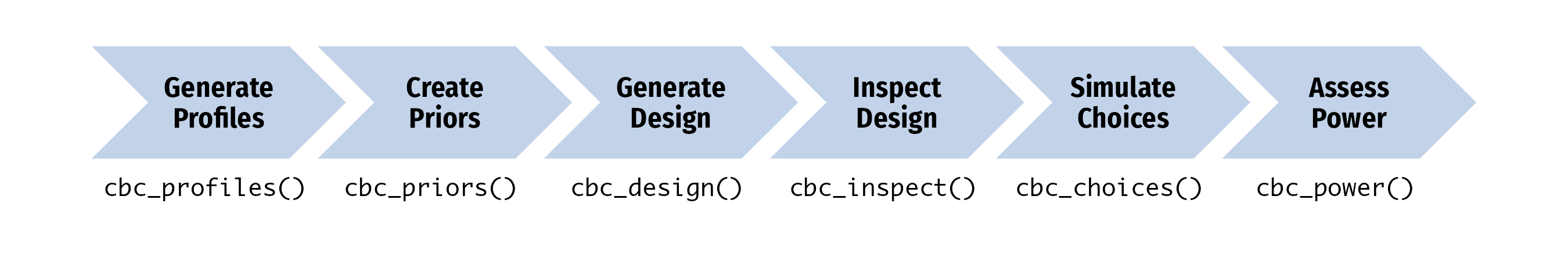
Each step uses functions that begin with cbc_ and builds on the previous step:

1. Generate Profiles → cbc_profiles() - Define attributes and levels
2. Specify Priors → cbc_priors() - Specify prior preference assumptions (optional)
3. Generate Designs → cbc_design() - Create choice question design
4. Inspect Designs → cbc_inspect() - Evaluate design quality
5. Simulate Choices → cbc_choices() - Generate realistic choice data
6. Assess Power → cbc_power() - Determine sample size requirements

Let's walk through each step with a complete example. Imagine we're designing a choice experiment to understand consumer preferences for apples. We want to study how price, type, and freshness influence purchase decisions.

Step 1: Generate Profiles

Start by defining the attributes and levels for your experiment:

profiles <- cbc_profiles(
  price = c(1.0, 1.5, 2.0, 2.5, 3.0), # Price per pound ($)
  type = c('Fuji', 'Gala', 'Honeycrisp'),
  freshness = c('Poor', 'Average', 'Excellent')
)

profiles

This creates all possible combinations of attribute levels - our "universe" of possible products to include in choice questions.

See the Generating Profiles article for more details and options on defining profiles, such as including restrictions.

Step 2: Specify Priors

Specify your assumptions about consumer preferences based on theory, literature, or pilot studies. These can be used for generating designs that incorporate these expected preferences as well as simulating choices for a given design.

priors <- cbc_priors(
  profiles = profiles,
  price = -0.25, # Negative = people prefer lower prices
  type = c(0.5, 1), # Gala and Honeycrisp preferred over Fuji (reference)
  freshness = c(0.6, 1.2) # Average and Excellent preferred over Poor (reference)
)

priors

Understanding Reference Levels

For categorical attributes, the reference level is set by the first level defined in cbc_profiles(), which in this case is "Fuji" for Type and "Poor" for Freshness. This would imply the following for the above set of priors:

• Type: Fuji (reference), Gala (+0.5), Honeycrisp (+1.0)
• Freshness: Poor (reference), Average (+0.6), Excellent (+1.2)

See the Specifying Priors article for more details and options on defining priors.

Step 3: Generate Designs

Create the set of choice questions that respondents will see. By default, all categorical variables are dummy-coded in the resulting design (you can convert the design back to categorical formatting with cbc_decode()):

design <- cbc_design(
  profiles = profiles,
  method = "stochastic", # D-optimal method
  n_alts = 3, # 2 alternatives per choice question
  n_q = 6, # 6 questions per respondent
  n_resp = 300, # 300 respondents
  priors = priors # Use our priors for optimization
)

design

The design generated is sufficient for a full survey for n_resp respondents. cbcTools offers several design methods, each with their own trade-offs:

• "random": Random profiles for each respondent.
• "shortcut": Frequency-balanced, often results in minimal overlap within choice questions.
• "minoverlap": Prioritizes minimizing attribute overlap within choice questions.
• "balanced": Optimizes both frequency balance and pairwise attribute interactions.
• "stochastic": Minimizes D-error by randomly swapping profiles.
• "modfed": Minimizes D-error by swapping out all possible profiles (slower, more thorough).
• "cea": Minimizes D-error by attribute-by-attribute swapping.

All design methods ensure:

1. No duplicate profiles within any choice set.
2. No duplicate choice sets within any respondent.
3. Dominance removal (if enabled) eliminates choice sets with dominant alternatives.

See the Generating Designs article for more details and options on generating experiment designs, such as including "no choice" options, using labeled designs, removing dominant options, and details about each design algorithm.

Step 4: Inspect Design

Use the cbc_inspect() function to evaluate the quality and properties of your design. Key things to look for:

• D-error: Lower values indicate more efficient designs
• Balance: Higher scores indicate better attribute level balance
• Overlap: Lower scores indicate less attribute overlap within questions
• Profile usage: Higher percentages indicate better use of available profiles

See cbc_inspect for more details.

cbc_inspect(design)

Step 5: Simulate Choices

Generate realistic choice data to test your design with the cbc_choices() function. By default, random choices are made, but if you provide priors with the priors argument, choices will be made according to the utility model defined by your priors:

# Simulate choices using our priors
choices <- cbc_choices(design, priors = priors)

choices

Taking a look at some quick summaries, you can see that the simulated choice patterns align with our priors - lower prices, preferred apple types, and better freshness should be chosen more often (not always for all levels though as there is some level of randomness involved). To do this, it's often easier to work with the design with categorical coding instead of dummy coding:

choices_cat <- cbc_decode(choices)

# Filter for the chosen rows only
choices_cat <- choices_cat[which(choices_cat$choice == 1), ]

# Counts of choices made for each attribute level
table(choices_cat$price)
table(choices_cat$type)
table(choices_cat$freshness)

See the Simulating Choices article for more details and options on inspeciting and comparing different experiment designs.

Step 6: Assess Power

Determine if your sample size provides adequate statistical power. The cbc_power() function auto-determines the attributes in your design and estimates multiple logit models using incrementally increasing sample sizes to assess power:

power <- cbc_power(choices)
power

You can easily visualize the results as well using the plot() function:

plot(power, type = "power", power_threshold = 0.9)

Finally, using the summary() function you can determine the exact size required to identify each attribute:

summary(power, power_threshold = 0.9)

See the Power article for more details and options on conducting power analyses to better understand your experiment designs.

Try the cbcTools package in your browser

library(cbcTools) help(cbcTools)

Run

Any scripts or data that you put into this service are public.

Nothing

cbcTools documentation built on Aug. 21, 2025, 6:03 p.m.