Data Collation"

In drhur: Learning R with Dr. Hu

knitr::opts_chunk$set(echo = TRUE,
                      message = FALSE,
                      warning = FALSE,
                      out.width="100%")

if (!require(pacman)) install.packages("pacman")

p_load(drhur,
       here,
       rio,
       tidyverse)
if (!require("dplyr")) {
  install.packages("dplyr")
  library("dplyr")
} else {
  library("dplyr")
}

Key Points

• Research Question:
• There are several survey data covering different regions, including: Afrobarometer, Asian Barometer and Latino Barómetro. If you want to create a global political barometer survey data, how should should you combine the data sets of different regions ?(hint: line merge)

• There are two data sets: Data set 1: Survey data on the perceptive inequality in various provinces in China Data set 2: Annual intra-provincial income gap data for each province If you want to study the impact of intra-provincial income gap on residents' inequality perception, how should you merge these two data sets? (hint: index merge, with the province and year as the index)

• Single Data Collation

  • explore
  • comb
  • filter
  • revise
• Multiple Data Collation
  • direct merge
  • index merge

Sample Data

{height=400}

We demonstrate this from a sample of the seventh wave of data (WVS7) from the [World Values Survey] (https://www.worldvaluessurvey.org/wvs.jsp), founded by the late political science professor Ronald Inglehart. This sample is 2% of the data in WVS7 and contains 24 variables. Specific variable information can be viewed through ?drhur::wvs7.

Data Exploration

Data exploration refers to the preliminary understanding of the data composition, structure, form, and content of unfamiliar data. It is the first step and a key step in data analysis.

Overview Raw Data

wvs7

• Tidy data（tibble）
  • row: observation unit
  • column: variable
  • unit: value

Understand Data Structures

• observations
• Variable name and number of variables
• data structure

wvs7

nrow(wvs7) # get the number of rows of data set
ncol(wvs7) # get the number of columns of data set
names(wvs7) # get variable name/column name
str(wvs7) # get variable name, variable name type, number of rows, number of columns

Variable Extraction

To discuss variable characteristics based on data, we must understand how to express the affiliation relationship between data and variables.

OOP systems including R are very good at multi-data and multi-variable collaborative use and analysis.

In other words, unlike some common data analysis software, R can load and combine multiple data at the same time - as long as they are stored in different objects.

wvs7[, "country"]

wvs7$country

Variable Features

The variable information extraction is exactly the same as the vector information extraction in the previous section.

We can also obtain variable distributions through the table command, and common variable information through the summary command.

Of course, R also supports obtaining the sum, mean, median, minimum, maximum, variance, IQR, etc. of the age variable. We will discuss these methods in detail in the next section.

table(wvs7$age)
summary(wvs7$age)

For non-numeric variables, we can obtain their information in the form of a summary table.

table(wvs7$female)
table(wvs7$marital)

For factor-based variables, we can also extract their hierarchical information.

levels(wvs7$religious)
levels(wvs7$marital)

Variable Characteristics

Variables may have different characteristics due to their classes, for example, class vectors cannot be averaged, so mean is meaningless for them.

But all variables have some attribute characteristics, such as variable length, category, feature value, etc.

The extraction commands for these features are also common.

length(wvs7$age) # get the length of the year (here is the number of rows)
unique(wvs7$age)

summary(wvs7$age) #get all the above information of the year
class(wvs7$age) #view year structure: vector, matrix, array, dataframe, list
typeof(wvs7$age) #view the year element type

Variable Overview

summary(wvs7$age)
summary(wvs7)

Data Combing

If data exploration is to look at variables from data, then data combing is to use variables as an index to understand data.

Considering the practicality, here we directly introduce how to use tidyverse for data combing.

But in fact, most of the data combing can be done through R's own statements.

We also place the actions of the own statement for the same task in the "Hint" unit.

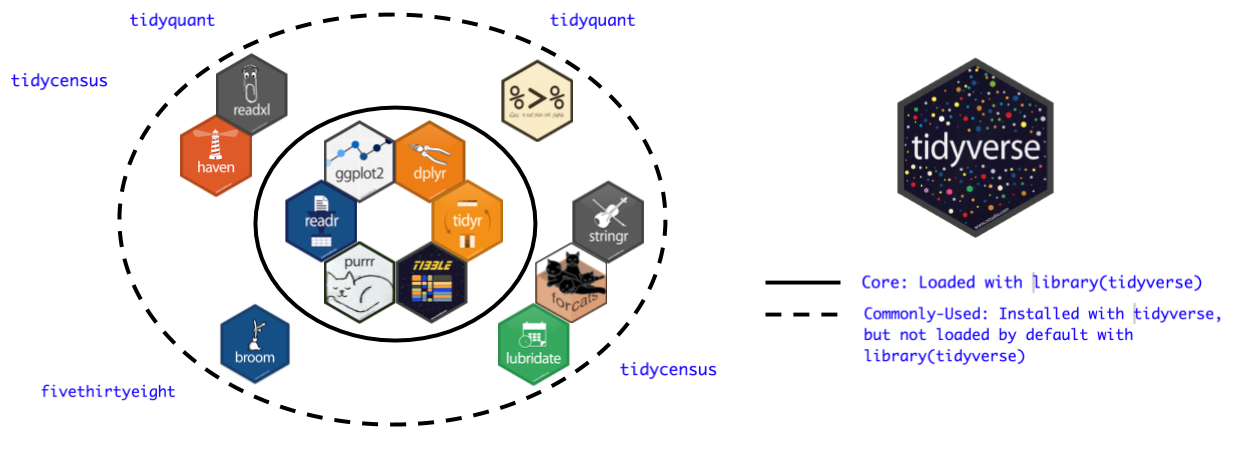
Let me introduce the tidyverse

• is an R package
• is a bunch of R packages!
• Like the Marvel and DC comics universes, all tidyverse members work in the same data structure and can talk to each other and use it together.

{height=300}

Package Installation

install.packages("tidyverse")
library("tidyverse")

dplyr Package

The component in tidyverse is responsible for data cleaning, and implements the style of doing one thing with one function.

Pipe

Before introducing the main commands of dplyr , we must first explain the pipe. Pipe can be expressed directly in R using |>, and %>% which is more powerful can also be used after calling dplyr.

The examples that follow use the latter.

In R, the Pipe is used to connect continuous actions for the same object, which is equivalent to "scraping" a continuous skill in an action game.

{height=400}

On the other hand, channels can also make the arrangement of each command more clear and easy to read.

To give another example, if we use code to simulate the whole process of cooking dumplings, it will roughly look like this:

eat_dumpling <- 
eat(
  dip(
    cook(
      fill(
        mix(
          meat, 
          with = c(salt, soy_sauce, green_onion, ginger)
          ), 
        with = wrapper
        ), 
      in = boilled_water
      ), 
    in = vinegar)
  )

After using the pipe, it can be written like this:

eat_dumpling <- 
mix(meat, with = c(salt, soy_sauce, green_onion, ginger)) %>% 
  fill(with = wrapper) %>% 
  cook(in = boilled_water) %>% 
  dip(in = vinegar) %>% 
  eat

Shortcut keys for %>%:

• Ctrl + Shift + M (Win)
• Cmd + Shift + M (Mac)

Variable Selection

select(<data>, <var1>, <var2>, ...)

There are 24 variables in the data, and some interesting variables are listed in the back, which is not convenient to see. We want to see a data frame with only these variables, namely country, age, education, confidence_gov .

select(wvs7, country, age, education, confidence_gov)

# If we want to see all the variables starting with confidence, what else can we do but list them one by one?

select(wvs7, country, age, education, starts_with("confidence"))

ends_with and matches are similar to starts_with.

Pay attention to the third person singular form.😝

Deleting a variable can be done with -:

select(wvs7, -(country:education))

A derivative of the select function is rename, with the syntax new.name = old.name.

rename(wvs7, nationality = country)

Data Sorting

arrange(<data>,...)

For example, we are curious about the confidence of the youngest people in state institutions, as well as information such as their education level and income level.

select(wvs7, age, confidence_gov, education, incomeLevel)

select(wvs7, age, confidence_gov, education, incomeLevel) %>% 
  arrange(age)

How about the oldest group?

select(wvs7, age, confidence_gov, education, incomeLevel) %>% 
  arrange(desc(age))

## What if we wanted to know the youngest and most educated person?

select(wvs7, age, confidence_gov, education, incomeLevel) %>% 
  arrange(age, desc(education))

Variable Value Filtering

As mentioned earlier, select is a filter for database variables, and filter is a filter based on variable values.

Continuing with the example above, if we were curious about the confidence of the youngest cohort in America in state institutions and their education level and income level.

select(wvs7, age, confidence_gov, education, incomeLevel) %>% 
  arrange(age)

select(wvs7, age, confidence_gov, education, incomeLevel, country) %>% 
  filter(country == "United States") %>% 
  arrange(age)

select(wvs7, age, confidence_gov, education, incomeLevel, country) %>% 
  filter(country == "United States") %>% 
  filter(age == min(age, na.rm = TRUE))

Data Modification

In data analysis, we often need to adjust and reprocess the data, mutate can help you do this.

The word 'mutate' means 'to change or alter,' which implies that the function does not create something out of nothing, but rather transforms something that already exists.

If we care about the effect of education level on differences in income levels, we can create a proportional variable.

mutate(wvs7, ratio_incomeEdu = incomeLevel / (education + 1)) %>%
  select(country, incomeLevel, education, ratio_incomeEdu) %>%
  arrange(desc(ratio_incomeEdu))

# What if you want to convert `ratio_incomeEdu` into a percentage?

mutate(wvs7, 
       ratio_incomeEdu = incomeLevel / (education + 1),
       ratio_incomeEdu = as.numeric(ratio_incomeEdu) %>%
         scales::percent()) %>%
  select(country, ratio_incomeEdu)

Numeric Statistics

count is used to count based on data.

For example,count can be used to calculate the number of men and women in our data. ^[Such lists are very common in statistics such as censuses. ]

wvs7 %>%
  count(female)

# What if you want to know the number of men and women in different age groups?

wvs7 %>%
  count(age, female)

summarise is used to convert individual data into statistical data.
For example, if we want to obtain the average age and education level of the sample.

wvs7 %>%
  summarise(age = mean(age, na.rm = TRUE),
            edu = mean(education, na.rm = TRUE))

group_by makes grouping operations possible.

wvs7 %>%
  group_by(female) %>% 
  summarise(age = mean(age, na.rm = TRUE),
            edu = mean(education, na.rm = TRUE))

group_by actually builds a group index for the existing data, and all subsequent operations will be performed in groups.

The inverse of this command is ungroup.

Bonus

How can we fill in the missing x and combine y and z into one variable?

df_toy <- data.frame(x = sample(c(1:2, NA, NA, NA)),
                     y = c(1, 2, NA, NA, 5),
                     z = c(NA, NA, 3, 4, 5))

df_toy

df_toy %>%
  mutate(x = coalesce(x, 0L),
         yz = coalesce(y, z)) # Ta-da~~~

Principles of Data Collation

The above series of operations have a common feature, have you found it?

head(wvs7)

• Do not touch raw data.
• Be careful with object coverage.

wvs7 <- mutate(wvs7, female = as.numeric(female))

Data Integration

Direct Merge

The premise of direct merging is basically the same as that of matrix operations: only the numbers in the first column match the next row.

• Row merge: the number of columns equal (Is this requirement necessary?)
• Column Merge: Number of rows equal

Give an example respectively:

wvs7_us <- filter(wvs7, country == "United States")
wvs7_russia <- filter(wvs7, country == "Russia")

# Create a US-Russian data

bind_rows(wvs7_us, wvs7_russia)

# What happens when unequal columns and rows are merged?

# Try this
bind_rows(tibble(x = 1:3), tibble(y = 1:4))

wvs7_conf <- select(wvs7, starts_with("confidence"))
wvs7_trust <- select(wvs7, starts_with("trust"))

# create a confidence-trust data

bind_cols(wvs7_conf, wvs7_trust)

Index Merge

Index merging refers to merging data based on a shared index sequence (which can be any variable).

Let's create two sample data:

1. Individual-level equality cognition data;
2. Country-level data on demographic variables.

If wvs7_eq is survey data and wvs7_country is demographic data, our research needs to combine these two sets of data to analyze the relationship between individual-level and country-level variables.

wvs7_eq <- select(wvs7, country, starts_with("equal")) %>% 
  filter(country %in% unique(country)[1:2])

wvs7_country <- group_by(wvs7, country) %>% 
  summarise(across(female:education, mean, na.rm = TRUE)) %>% 
  ungroup %>% 
  filter(country %in% unique(country)[2:3])

inner_join(wvs7_eq, wvs7_country)
left_join(wvs7_eq, wvs7_country)
right_join(wvs7_eq, wvs7_country)
full_join(wvs7_eq, wvs7_country)

Summary

1. Think clearly before taking action ;
2. Use the dplyr function to neatly and comprehensively;
   • Explore: head, tail
     • structure: nrow, ncol, names, str
     • features: table, levels
     • properties: length, unique, summary, class, typeof
   • Combing: dplyr command set
3. Principle of data integration : do not touch the original data
4. Data Merging
   • direct merge: bind_*
   • Index merge: *_join

drhur documentation built on May 31, 2023, 6:03 p.m.