Nothing
Raincloud vignette
In ggrain: A Rainclouds Geom for 'ggplot2'
knitr::opts_chunk$set(
  collapse = TRUE,
  #warning = FALSE, message = FALSE,
  comment = "#>"
)
library(ggrain)
The geom_rain() function
- handles as many rainclouds as you wish and can overlap them by a group
- connects within-subject observations longitudinally with lines using
id.long.var argument
- colors dots by a covariate using the
cov argument
- handles likert data by adding y-jittering with
likert = TRUE
- changes orientation with
+ coord_flip()
All individual elements of the plots can be edited, these are split into aesthetic and positioning arguments that are supplied by lists. For example the boxplots can be edited with boxplot.args and boxplot.args.pos, yet the others can also be edited by substituting for their name, i.e. point/violin/line. When you supply a list the defaults are overwritten so you may need to re-add them. To see the defaults run ?geom_rain.
Introduction
Here is our first plot which is just simply all the values of Sepal.Width in the iris dataset. For the function to work the value you want to plot must be given to the y argument in ggplot. You can then flip the plot with + coord_flip() as we demonstrate below.
ggplot(iris, aes(1, Sepal.Width)) +
  geom_rain() +
  theme_classic() +
  theme(axis.title.x = element_blank(),
        axis.text.x = element_blank(), axis.ticks.x = element_blank())
Let's see what is happening over the 3 Species of flowers. The fill must be a factor or a character vector!
ggplot(iris, aes(1, Sepal.Width, fill = Species)) +
  geom_rain(alpha = .5) +
  theme_classic() +
  scale_fill_brewer(palette = 'Dark2')
Let's color the dots by Species, we do this by adding color = Species to ggplot. The default behavior of geom_boxplot is to color the lines in the boxplot showing the median and IQR. Therefore, we need to add a boxplot.args list to re-color the boxplot to black. When we do this all defaults are lost therefore we must add the options to not show outliers.
ggplot(iris, aes(1, Sepal.Width, fill = Species, color = Species)) +
  geom_rain(alpha = .6,
            boxplot.args = list(color = "black", outlier.shape = NA)) +
  theme_classic() +
  scale_fill_brewer(palette = 'Dark2') +
  scale_color_brewer(palette = 'Dark2')
It is also possible to nudge the box plots so they are not overlapping with boxplot.args.pos. We will also flip them by setting the rain.side argument to left (i.e., 'l').
ggplot(iris, aes(1, Sepal.Width, fill = Species, color = Species)) +
  geom_rain(alpha = .5, rain.side = 'l',
            boxplot.args = list(color = "black", outlier.shape = NA),
            boxplot.args.pos = list(
              position = ggpp::position_dodgenudge(x = .1, width = 0.1), width = 0.1
            )) +
  theme_classic() +
  scale_fill_brewer(palette = 'Dark2') +
  scale_color_brewer(palette = 'Dark2') +
  guides(fill = 'none', color = 'none')
It could be even more useful to see the different species of flowers side by side rather than overlapping. The y value must be a factor or a character vector!
ggplot(iris, aes(Species, Sepal.Width, fill = Species)) +
  geom_rain(alpha = .5) +
  theme_classic() +
  scale_fill_brewer(palette = 'Dark2') +
  guides(fill = 'none', color = 'none')
We can flip the plots by adding coord_flip().
ggplot(iris, aes(Species, Sepal.Width, fill = Species)) +
  geom_rain(alpha = .5) +
  theme_classic() +
  scale_fill_brewer(palette = 'Dark2') +
  guides(fill = 'none', color = 'none') +
  coord_flip()
This plot is a bit crammed, lets spread stuff out using the boxplot.args.pos & violin.args.pos arguments.
ggplot(iris, aes(Species, Sepal.Width, fill = Species)) +
  geom_rain(alpha = .5,
            boxplot.args.pos = list(
              width = 0.05, position = position_nudge(x = 0.13)),
            violin.args.pos = list(
              side = "r",
              width = 0.7, position = position_nudge(x = 0.2))) +
  theme_classic() +
  scale_fill_brewer(palette = 'Dark2') +
  guides(fill = 'none', color = 'none') +
  coord_flip()
Instead of coloring the dots by Species, the package offers the ability to color to another variable such as Sepal.Length. This will allow us to visualize how Sepal.Width and Sepal.Length relate to each other in each Species of flower.
We can do this by adding them as a covariate with the cov argument. At the current time the argument must be given as a string.
ggplot(iris, aes(Species, Sepal.Width, fill = Species)) +
  geom_rain(alpha = .6,
            cov = "Sepal.Length") +
  theme_classic() +
  scale_fill_brewer(palette = 'Dark2') +
  guides(fill = 'none', color = 'none') +
  scale_color_viridis_c(option =  "A", direction = -1)
We will now take the species versicolor and virginica and make longitudinal data. We are going to see what fertilizer does to the Sepal.Width of both species!
set.seed(42) # the magic number

iris_subset <- iris[iris$Species %in% c('versicolor', 'virginica'),]

iris.long <- cbind(rbind(iris_subset, iris_subset, iris_subset),
                   data.frame(time = c(rep("t1", dim(iris_subset)[1]), rep("t2", dim(iris_subset)[1]), rep("t3", dim(iris_subset)[1])),
                              id = c(rep(1:dim(iris_subset)[1]), rep(1:dim(iris_subset)[1]), rep(1:dim(iris_subset)[1]))))

# adding .5 and some noise to the versicolor species in t2
iris.long$Sepal.Width[iris.long$Species == 'versicolor' & iris.long$time == "t2"] <- iris.long$Sepal.Width[iris.long$Species == 'versicolor' & iris.long$time == "t2"] + .5 + rnorm(length(iris.long$Sepal.Width[iris.long$Species == 'versicolor' & iris.long$time == "t2"]), sd = .2)
# adding .8 and some noise to the versicolor species in t3
iris.long$Sepal.Width[iris.long$Species == 'versicolor' & iris.long$time == "t3"] <- iris.long$Sepal.Width[iris.long$Species == 'versicolor' & iris.long$time == "t3"] + .8 + rnorm(length(iris.long$Sepal.Width[iris.long$Species == 'versicolor' & iris.long$time == "t3"]), sd = .2)

# now we subtract -.2 and some noise to the virginica species
iris.long$Sepal.Width[iris.long$Species == 'virginica' & iris.long$time == "t2"] <- iris.long$Sepal.Width[iris.long$Species == 'virginica' & iris.long$time == "t2"] - .2 + rnorm(length(iris.long$Sepal.Width[iris.long$Species == 'virginica' & iris.long$time == "t2"]), sd = .2)

# now we subtract -.4 and some noise to the virginica species
iris.long$Sepal.Width[iris.long$Species == 'virginica' & iris.long$time == "t3"] <- iris.long$Sepal.Width[iris.long$Species == 'virginica' & iris.long$time == "t3"] - .4 + rnorm(length(iris.long$Sepal.Width[iris.long$Species == 'virginica' & iris.long$time == "t3"]), sd = .2)

iris.long$Sepal.Width <- round(iris.long$Sepal.Width, 1) # rounding Sepal.Width so t2 data is on the same resolution
iris.long$time <- factor(iris.long$time, levels = c('t1', 't2', 't3'))
Here we plot the species overlapping at each time point. We can see fertilizer caused the Sepal Width of the versicolor species to increase while the virginica species decreased slightly!
ggplot(iris.long[iris.long$time %in% c('t1', 't2'),], aes(time, Sepal.Width, fill = Species)) +
  geom_rain(alpha = .5) +
  theme_classic() +
  scale_fill_manual(values=c("dodgerblue", "darkorange")) +
  guides(fill = 'none', color = 'none')
We can easily flank them using the rain.side argument for 2-by-2 flanking (i.e., 'f2x2'). This also automatically uses ggpp::position_dodgenudge to dodge the boxplots. Yet, for descriptive purposes with will use the flanking argument rain.side = 'f' with the defaults from 'f2x2'. The rain.side = 'f' argument defaults to a 2-by-2 yet throw a warning if you don't remap the violin.args.pos. When using flanking with more groups or more time points you must give specific boxplot.args.pos and violin.args.pos for each element. The left elements must have negative x-axis nudging values with the right ones have positive x-axis nudging values.
ggplot(iris.long[iris.long$time %in% c('t1', 't2'),], aes(time, Sepal.Width, fill = Species)) +
  geom_rain(alpha = .5, rain.side = 'f',
             boxplot.args.pos = list(width = .1,
                position = ggpp::position_dodgenudge(width = .1, #width needed now in ggpp version 0.5.g
                  x = c(-.13, -.13, # pre versicolor, pre virginica
                        .13, .13))), # post; post
            violin.args.pos = list(width = .7,
             position = position_nudge(x = c(rep(-.2, 256*2), rep(-.2, 256*2),# pre; pre
                                             rep(.2, 256*2), rep(.2, 256*2))))) + #post; post
  theme_classic() +
  scale_fill_manual(values=c("dodgerblue", "darkorange")) +
  guides(fill = 'none', color = 'none')
We can connect each plant with lines using the id.long.var argument, we will also use the convient rain.side = 'f2x2'. As with the cov argument, it must be a string linking the ids of each observation across time.
ggplot(iris.long[iris.long$time %in% c('t1', 't2'),], aes(time, Sepal.Width, fill = Species)) +
  geom_rain(alpha = .5, rain.side = 'f2x2', id.long.var = "id") +
  theme_classic() +
  scale_fill_manual(values=c("dodgerblue", "darkorange")) +
  guides(fill = 'none', color = 'none')
We can color the dots and the connecting lines by Species! We will also remove the lines around the violins by specifying their color = NA, yet we now must re-add the alpha argument.
ggplot(iris.long[iris.long$time %in% c('t1', 't2'),], aes(time, Sepal.Width, fill = Species, color = Species)) +
  geom_rain(alpha = .5, rain.side = 'f2x2', id.long.var = "id",
            violin.args = list(color = NA, alpha = .7)) +
  theme_classic() +
  scale_fill_manual(values=c("dodgerblue", "darkorange")) +
  scale_color_manual(values=c("dodgerblue", "darkorange")) +
  guides(fill = 'none', color = 'none')
We can start to combine aspects, for example here is three timepoints with subjects connected, special flanking and a covariate mapped!
ggplot(iris.long, aes(time, Sepal.Width, fill = Species)) +
  geom_rain(alpha = .5, rain.side = 'f', id.long.var = "id", cov = "Sepal.Length",
            boxplot.args = list(outlier.shape = NA, alpha = .8),
            violin.args = list(alpha = .8, color = NA),
            boxplot.args.pos = list(width = .1,
             position = ggpp::position_dodgenudge(width = .1,
                                                  x = c(-.13, -.13, # t1 old, t1 young
                                                        -.13, .13,
                                                         .13, .13))),
            violin.args.pos = list(width = .7,
             position = position_nudge(x = c(rep(-.2, 256*2), rep(-.2, 256*2),# t1
                                             rep(-.2, 256*2), rep(.2, 256*2), # t2
                                             rep(.2, 256*2), rep(.2, 256*2))))) +
  theme_classic() +
  scale_fill_manual(values=c("dodgerblue", "darkorange")) +
  scale_color_viridis_c(option =  "A", direction = -1) +
  guides(fill = 'none', color = 'none')
Lastly, we can add a mean trend line using stat_summary. Accentuating the opposite effects fertilizers had on the two species of flowers!
ggplot(iris.long[iris.long$time %in% c('t1', 't2'),], aes(time, Sepal.Width, fill = Species)) +
  geom_rain(alpha = .5, rain.side = 'f2x2') +
  theme_classic() +
  stat_summary(fun = mean, geom = "line", aes(group = Species, color = Species)) +
  stat_summary(fun = mean, geom = "point",
               aes(group = Species, color = Species)) +
  scale_fill_manual(values=c("dodgerblue", "darkorange")) +
  scale_color_manual(values=c("dodgerblue", "darkorange")) +
  guides(fill = 'none', color = 'none')
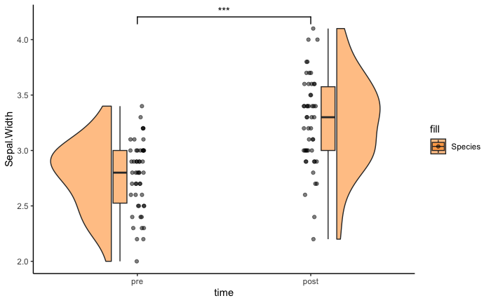
Here is some sample code on how to do a significance test on a 1-by-1 flanking raincloud with the package ggsignif. We will not run it as we don't want to add ggsignif as a package dependency.
ggplot(iris.long[iris.long$Species == 'versicolor' & iris.long$time %in% c('t1', 't2'),], aes(time, Sepal.Width, fill = Species)) +
  geom_rain(alpha = .5, rain.side = 'f1x1') +
 ggsignif::geom_signif(
  comparisons = list(c("t1", "t2")),
  map_signif_level = TRUE) +
scale_fill_manual(values=c("darkorange", "darkorange")) +
theme_classic()
Try the ggrain package in your browser
Any scripts or data that you put into this service are public.
ggrain documentation built on May 29, 2024, 7:24 a.m.
R Package Documentation
Browse R Packages
We want your feedback!
Note that we can't provide technical support on individual packages. You should contact the package authors for that.
knitr::opts_chunk$set( collapse = TRUE, #warning = FALSE, message = FALSE, comment = "#>" )
library(ggrain)
The geom_rain() function
- handles as many rainclouds as you wish and can overlap them by a group
- connects within-subject observations longitudinally with lines using
id.long.varargument - colors dots by a covariate using the
covargument - handles likert data by adding y-jittering with
likert = TRUE - changes orientation with
+ coord_flip()
All individual elements of the plots can be edited, these are split into aesthetic and positioning arguments that are supplied by lists. For example the boxplots can be edited with boxplot.args and boxplot.args.pos, yet the others can also be edited by substituting for their name, i.e. point/violin/line. When you supply a list the defaults are overwritten so you may need to re-add them. To see the defaults run ?geom_rain.
Introduction
Here is our first plot which is just simply all the values of Sepal.Width in the iris dataset. For the function to work the value you want to plot must be given to the y argument in ggplot. You can then flip the plot with + coord_flip() as we demonstrate below.
ggplot(iris, aes(1, Sepal.Width)) + geom_rain() + theme_classic() + theme(axis.title.x = element_blank(), axis.text.x = element_blank(), axis.ticks.x = element_blank())
Let's see what is happening over the 3 Species of flowers. The fill must be a factor or a character vector!
ggplot(iris, aes(1, Sepal.Width, fill = Species)) + geom_rain(alpha = .5) + theme_classic() + scale_fill_brewer(palette = 'Dark2')
Let's color the dots by Species, we do this by adding color = Species to ggplot. The default behavior of geom_boxplot is to color the lines in the boxplot showing the median and IQR. Therefore, we need to add a boxplot.args list to re-color the boxplot to black. When we do this all defaults are lost therefore we must add the options to not show outliers.
ggplot(iris, aes(1, Sepal.Width, fill = Species, color = Species)) + geom_rain(alpha = .6, boxplot.args = list(color = "black", outlier.shape = NA)) + theme_classic() + scale_fill_brewer(palette = 'Dark2') + scale_color_brewer(palette = 'Dark2')
It is also possible to nudge the box plots so they are not overlapping with boxplot.args.pos. We will also flip them by setting the rain.side argument to left (i.e., 'l').
ggplot(iris, aes(1, Sepal.Width, fill = Species, color = Species)) + geom_rain(alpha = .5, rain.side = 'l', boxplot.args = list(color = "black", outlier.shape = NA), boxplot.args.pos = list( position = ggpp::position_dodgenudge(x = .1, width = 0.1), width = 0.1 )) + theme_classic() + scale_fill_brewer(palette = 'Dark2') + scale_color_brewer(palette = 'Dark2') + guides(fill = 'none', color = 'none')
It could be even more useful to see the different species of flowers side by side rather than overlapping. The y value must be a factor or a character vector!
ggplot(iris, aes(Species, Sepal.Width, fill = Species)) + geom_rain(alpha = .5) + theme_classic() + scale_fill_brewer(palette = 'Dark2') + guides(fill = 'none', color = 'none')
We can flip the plots by adding coord_flip().
ggplot(iris, aes(Species, Sepal.Width, fill = Species)) + geom_rain(alpha = .5) + theme_classic() + scale_fill_brewer(palette = 'Dark2') + guides(fill = 'none', color = 'none') + coord_flip()
This plot is a bit crammed, lets spread stuff out using the boxplot.args.pos & violin.args.pos arguments.
ggplot(iris, aes(Species, Sepal.Width, fill = Species)) + geom_rain(alpha = .5, boxplot.args.pos = list( width = 0.05, position = position_nudge(x = 0.13)), violin.args.pos = list( side = "r", width = 0.7, position = position_nudge(x = 0.2))) + theme_classic() + scale_fill_brewer(palette = 'Dark2') + guides(fill = 'none', color = 'none') + coord_flip()
Instead of coloring the dots by Species, the package offers the ability to color to another variable such as Sepal.Length. This will allow us to visualize how Sepal.Width and Sepal.Length relate to each other in each Species of flower.
We can do this by adding them as a covariate with the cov argument. At the current time the argument must be given as a string.
ggplot(iris, aes(Species, Sepal.Width, fill = Species)) + geom_rain(alpha = .6, cov = "Sepal.Length") + theme_classic() + scale_fill_brewer(palette = 'Dark2') + guides(fill = 'none', color = 'none') + scale_color_viridis_c(option = "A", direction = -1)
We will now take the species versicolor and virginica and make longitudinal data. We are going to see what fertilizer does to the Sepal.Width of both species!
set.seed(42) # the magic number iris_subset <- iris[iris$Species %in% c('versicolor', 'virginica'),] iris.long <- cbind(rbind(iris_subset, iris_subset, iris_subset), data.frame(time = c(rep("t1", dim(iris_subset)[1]), rep("t2", dim(iris_subset)[1]), rep("t3", dim(iris_subset)[1])), id = c(rep(1:dim(iris_subset)[1]), rep(1:dim(iris_subset)[1]), rep(1:dim(iris_subset)[1])))) # adding .5 and some noise to the versicolor species in t2 iris.long$Sepal.Width[iris.long$Species == 'versicolor' & iris.long$time == "t2"] <- iris.long$Sepal.Width[iris.long$Species == 'versicolor' & iris.long$time == "t2"] + .5 + rnorm(length(iris.long$Sepal.Width[iris.long$Species == 'versicolor' & iris.long$time == "t2"]), sd = .2) # adding .8 and some noise to the versicolor species in t3 iris.long$Sepal.Width[iris.long$Species == 'versicolor' & iris.long$time == "t3"] <- iris.long$Sepal.Width[iris.long$Species == 'versicolor' & iris.long$time == "t3"] + .8 + rnorm(length(iris.long$Sepal.Width[iris.long$Species == 'versicolor' & iris.long$time == "t3"]), sd = .2) # now we subtract -.2 and some noise to the virginica species iris.long$Sepal.Width[iris.long$Species == 'virginica' & iris.long$time == "t2"] <- iris.long$Sepal.Width[iris.long$Species == 'virginica' & iris.long$time == "t2"] - .2 + rnorm(length(iris.long$Sepal.Width[iris.long$Species == 'virginica' & iris.long$time == "t2"]), sd = .2) # now we subtract -.4 and some noise to the virginica species iris.long$Sepal.Width[iris.long$Species == 'virginica' & iris.long$time == "t3"] <- iris.long$Sepal.Width[iris.long$Species == 'virginica' & iris.long$time == "t3"] - .4 + rnorm(length(iris.long$Sepal.Width[iris.long$Species == 'virginica' & iris.long$time == "t3"]), sd = .2) iris.long$Sepal.Width <- round(iris.long$Sepal.Width, 1) # rounding Sepal.Width so t2 data is on the same resolution iris.long$time <- factor(iris.long$time, levels = c('t1', 't2', 't3'))
Here we plot the species overlapping at each time point. We can see fertilizer caused the Sepal Width of the versicolor species to increase while the virginica species decreased slightly!
ggplot(iris.long[iris.long$time %in% c('t1', 't2'),], aes(time, Sepal.Width, fill = Species)) + geom_rain(alpha = .5) + theme_classic() + scale_fill_manual(values=c("dodgerblue", "darkorange")) + guides(fill = 'none', color = 'none')
We can easily flank them using the rain.side argument for 2-by-2 flanking (i.e., 'f2x2'). This also automatically uses ggpp::position_dodgenudge to dodge the boxplots. Yet, for descriptive purposes with will use the flanking argument rain.side = 'f' with the defaults from 'f2x2'. The rain.side = 'f' argument defaults to a 2-by-2 yet throw a warning if you don't remap the violin.args.pos. When using flanking with more groups or more time points you must give specific boxplot.args.pos and violin.args.pos for each element. The left elements must have negative x-axis nudging values with the right ones have positive x-axis nudging values.
ggplot(iris.long[iris.long$time %in% c('t1', 't2'),], aes(time, Sepal.Width, fill = Species)) + geom_rain(alpha = .5, rain.side = 'f', boxplot.args.pos = list(width = .1, position = ggpp::position_dodgenudge(width = .1, #width needed now in ggpp version 0.5.g x = c(-.13, -.13, # pre versicolor, pre virginica .13, .13))), # post; post violin.args.pos = list(width = .7, position = position_nudge(x = c(rep(-.2, 256*2), rep(-.2, 256*2),# pre; pre rep(.2, 256*2), rep(.2, 256*2))))) + #post; post theme_classic() + scale_fill_manual(values=c("dodgerblue", "darkorange")) + guides(fill = 'none', color = 'none')
We can connect each plant with lines using the id.long.var argument, we will also use the convient rain.side = 'f2x2'. As with the cov argument, it must be a string linking the ids of each observation across time.
ggplot(iris.long[iris.long$time %in% c('t1', 't2'),], aes(time, Sepal.Width, fill = Species)) + geom_rain(alpha = .5, rain.side = 'f2x2', id.long.var = "id") + theme_classic() + scale_fill_manual(values=c("dodgerblue", "darkorange")) + guides(fill = 'none', color = 'none')
We can color the dots and the connecting lines by Species! We will also remove the lines around the violins by specifying their color = NA, yet we now must re-add the alpha argument.
ggplot(iris.long[iris.long$time %in% c('t1', 't2'),], aes(time, Sepal.Width, fill = Species, color = Species)) + geom_rain(alpha = .5, rain.side = 'f2x2', id.long.var = "id", violin.args = list(color = NA, alpha = .7)) + theme_classic() + scale_fill_manual(values=c("dodgerblue", "darkorange")) + scale_color_manual(values=c("dodgerblue", "darkorange")) + guides(fill = 'none', color = 'none')
We can start to combine aspects, for example here is three timepoints with subjects connected, special flanking and a covariate mapped!
ggplot(iris.long, aes(time, Sepal.Width, fill = Species)) + geom_rain(alpha = .5, rain.side = 'f', id.long.var = "id", cov = "Sepal.Length", boxplot.args = list(outlier.shape = NA, alpha = .8), violin.args = list(alpha = .8, color = NA), boxplot.args.pos = list(width = .1, position = ggpp::position_dodgenudge(width = .1, x = c(-.13, -.13, # t1 old, t1 young -.13, .13, .13, .13))), violin.args.pos = list(width = .7, position = position_nudge(x = c(rep(-.2, 256*2), rep(-.2, 256*2),# t1 rep(-.2, 256*2), rep(.2, 256*2), # t2 rep(.2, 256*2), rep(.2, 256*2))))) + theme_classic() + scale_fill_manual(values=c("dodgerblue", "darkorange")) + scale_color_viridis_c(option = "A", direction = -1) + guides(fill = 'none', color = 'none')
Lastly, we can add a mean trend line using stat_summary. Accentuating the opposite effects fertilizers had on the two species of flowers!
ggplot(iris.long[iris.long$time %in% c('t1', 't2'),], aes(time, Sepal.Width, fill = Species)) + geom_rain(alpha = .5, rain.side = 'f2x2') + theme_classic() + stat_summary(fun = mean, geom = "line", aes(group = Species, color = Species)) + stat_summary(fun = mean, geom = "point", aes(group = Species, color = Species)) + scale_fill_manual(values=c("dodgerblue", "darkorange")) + scale_color_manual(values=c("dodgerblue", "darkorange")) + guides(fill = 'none', color = 'none')
Here is some sample code on how to do a significance test on a 1-by-1 flanking raincloud with the package ggsignif. We will not run it as we don't want to add ggsignif as a package dependency.
ggplot(iris.long[iris.long$Species == 'versicolor' & iris.long$time %in% c('t1', 't2'),], aes(time, Sepal.Width, fill = Species)) + geom_rain(alpha = .5, rain.side = 'f1x1') + ggsignif::geom_signif( comparisons = list(c("t1", "t2")), map_signif_level = TRUE) + scale_fill_manual(values=c("darkorange", "darkorange")) + theme_classic()
Try the ggrain package in your browser
Any scripts or data that you put into this service are public.
R Package Documentation
Browse R Packages
We want your feedback!
Note that we can't provide technical support on individual packages. You should contact the package authors for that.
Embedding an R snippet on your website
Add the following code to your website.
For more information on customizing the embed code, read Embedding Snippets.