README.md

In giscoR: Download Map Data from GISCO API - Eurostat

giscoR

giscoR is an API package that helps to retrieve data from Eurostat - GISCO (the Geographic Information System of the COmmission). It also provides some lightweight data sets ready to use without downloading.

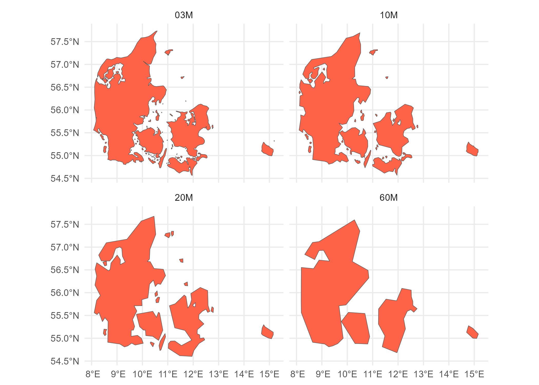
GISCO is a geospatial open data repository including several data sets as countries, coastal lines, labels or NUTS levels. The data sets are usually provided at several resolution levels (60M/20M/10M/03M/01M) and in 3 different projections (4326/3035/3857).

Note that the package does not provide metadata on the downloaded files, the information is available on the API webpage.

Full site with examples and vignettes on https://ropengov.github.io/giscoR/

Installation

Install giscoR from CRAN:

install.packages("giscoR")

You can install the developing version of giscoR with:

library(remotes)
install_github("rOpenGov/giscoR")

Alternatively, you can install giscoR using the r-universe:

install.packages("giscoR",
  repos = c("https://ropengov.r-universe.dev", "https://cloud.r-project.org")
)

Usage

This script highlights some features of giscoR:

library(giscoR)
library(sf)
library(dplyr)

# Different resolutions
DNK_res60 <- gisco_get_countries(resolution = "60", country = "DNK") %>%
  mutate(res = "60M")
DNK_res20 <-
  gisco_get_countries(resolution = "20", country = "DNK") %>%
  mutate(res = "20M")
DNK_res10 <-
  gisco_get_countries(resolution = "10", country = "DNK") %>%
  mutate(res = "10M")
DNK_res03 <-
  gisco_get_countries(resolution = "03", country = "DNK") %>%
  mutate(res = "03M")


DNK_all <- bind_rows(DNK_res60, DNK_res20, DNK_res10, DNK_res03)

# Plot ggplot2

library(ggplot2)

ggplot(DNK_all) +
  geom_sf(fill = "tomato") +
  facet_wrap(vars(res)) +
  theme_minimal()

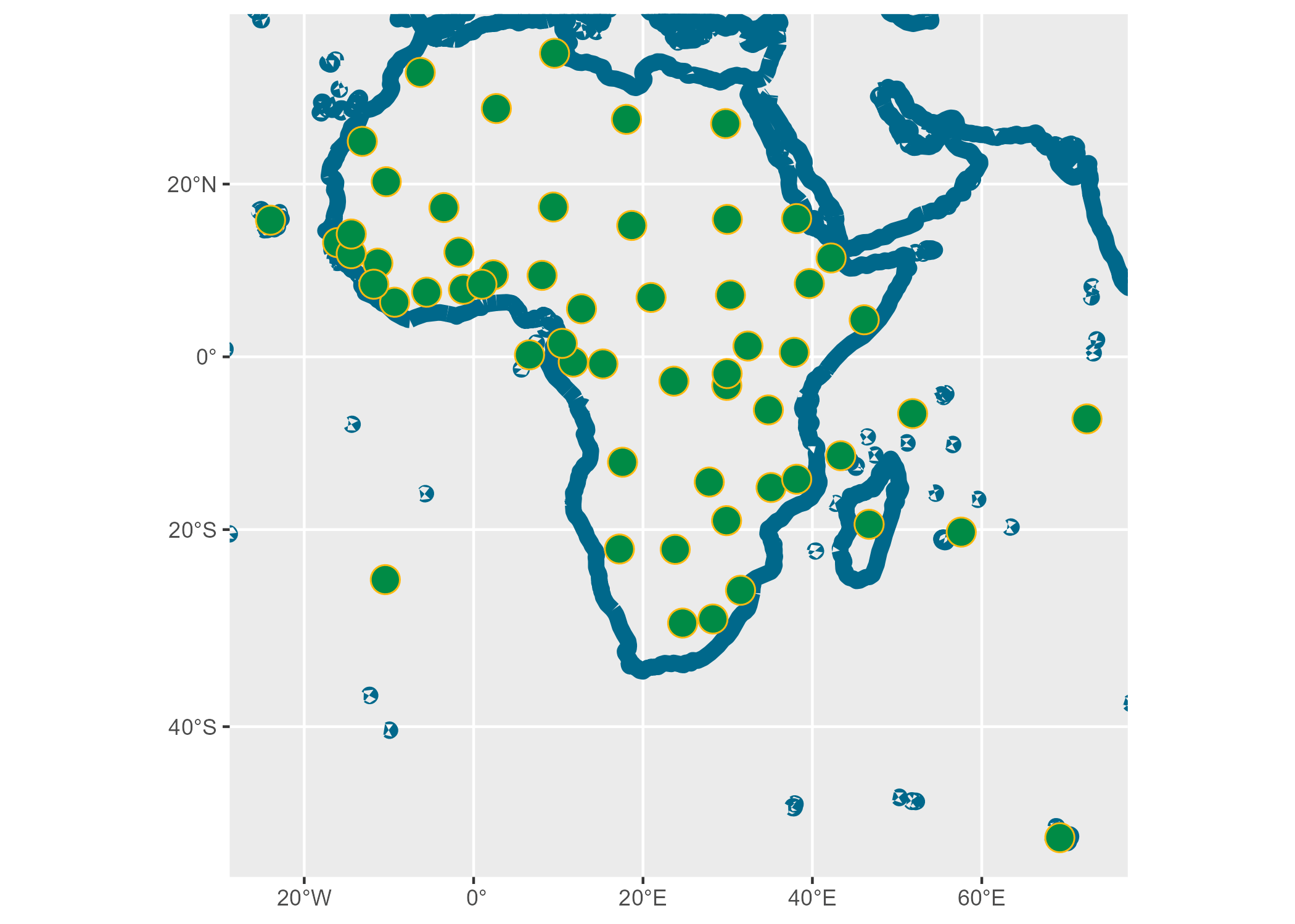
# Labels and Lines available

labs <- gisco_get_countries(
  spatialtype = "LB",
  region = "Africa",
  epsg = "3857"
)

coast <- gisco_get_countries(
  spatialtype = "COASTL",
  epsg = "3857"
)

# For zooming
afr_bbox <- st_bbox(labs)

ggplot(coast) +
  geom_sf(col = "deepskyblue4", linewidth = 3) +
  geom_sf(data = labs, fill = "springgreen4", col = "darkgoldenrod1", size = 5, shape = 21) +
  coord_sf(
    xlim = afr_bbox[c("xmin", "xmax")],
    ylim = afr_bbox[c("ymin", "ymax")]
  )

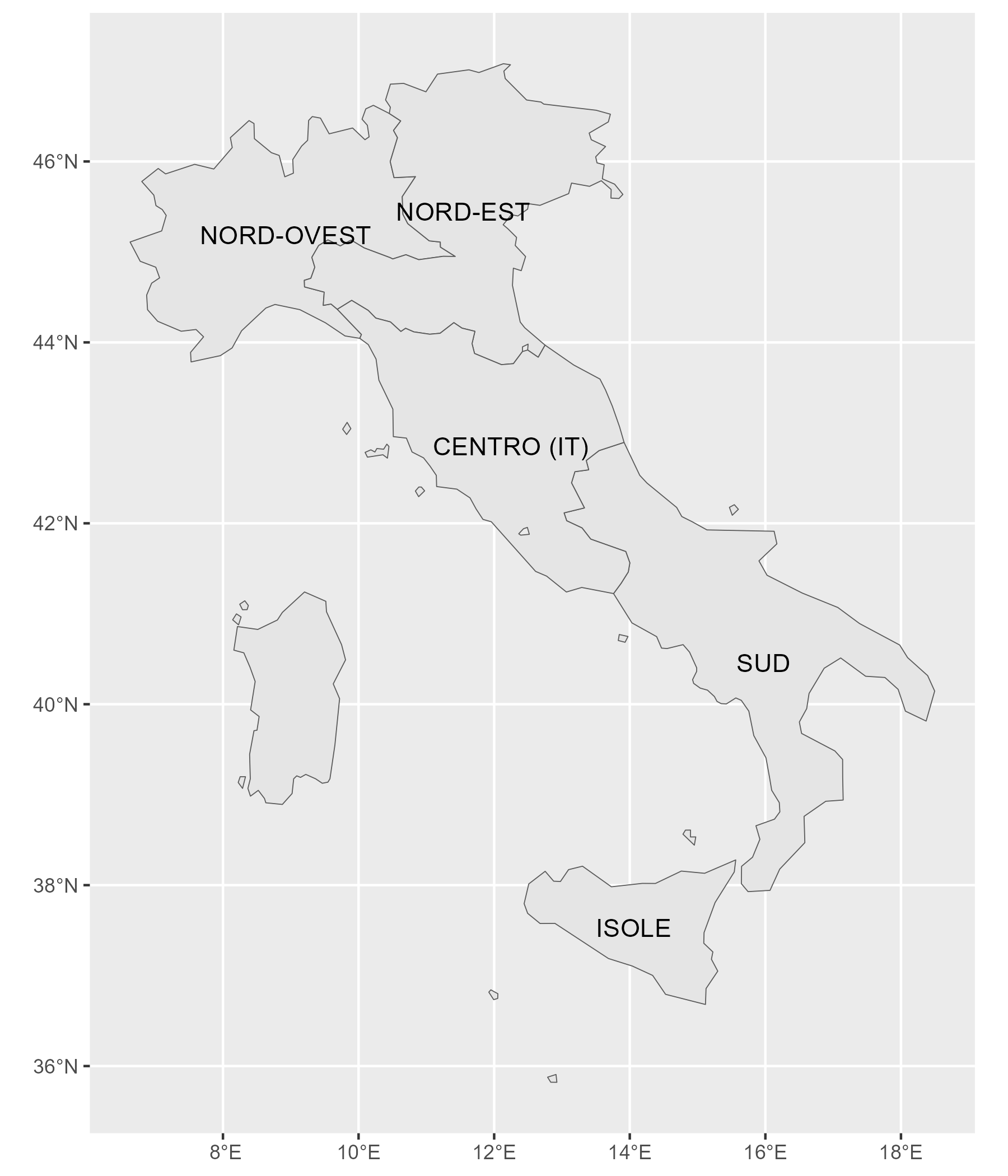
Labels

An example of a labeled map using ggplot2:

ITA <- gisco_get_nuts(country = "Italy", nuts_level = 1)

ggplot(ITA) +
  geom_sf() +
  geom_sf_text(aes(label = NAME_LATN)) +
  theme(axis.title = element_blank())

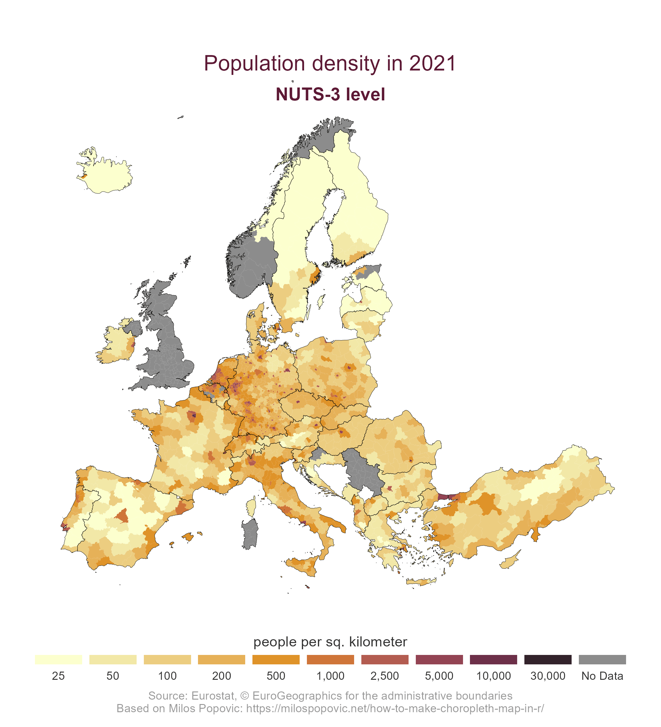
Thematic maps

An example of a thematic map plotted with the ggplot2 package. The information is extracted via the eurostat package. We would follow the fantastic approach presented by Milos Popovic on this post:

We start by extracting the corresponding geographic data:

# Get shapes
nuts3 <- gisco_get_nuts(
  year = "2016",
  epsg = "3035",
  resolution = "3",
  nuts_level = "3"
)

# Group by NUTS by country and convert to lines
country_lines <- nuts3 %>%
  group_by(
    CNTR_CODE
  ) %>%
  summarise(n = n()) %>%
  st_cast("MULTILINESTRING")

We now download the data from Eurostat:

# Use eurostat
library(eurostat)

popdens <- get_eurostat("demo_r_d3dens") %>%  filter(time == "2018-01-01")

By last, we merge and manipulate the data for creating the final plot:

# Merge data
nuts3.sf <- nuts3 %>%
  left_join(popdens, by = c("NUTS_ID" = "geo"))


# Breaks and labels

br <- c(0, 25, 50, 100, 200, 500, 1000, 2500, 5000, 10000, 30000)

nuts3.sf <- nuts3.sf %>%
  mutate(values_cut = cut(values, br, dig.lab = 5))

labs_plot <- prettyNum(br[-1], big.mark = ",")

# Palette
pal <- hcl.colors(length(br) - 1, "Lajolla")


# Plot

ggplot(nuts3.sf) +
  geom_sf(aes(fill = values_cut), linewidth = 0, color = NA, alpha = 0.9) +
  geom_sf(data = country_lines, col = "black", linewidth = 0.1) +
  # Center in Europe: EPSG 3035
  coord_sf(
    xlim = c(2377294, 7453440),
    ylim = c(1313597, 5628510)
  ) +
  labs(
    title = "Population density in 2018",
    subtitle = "NUTS-3 level",
    caption = paste0(
      "Source: Eurostat, ", gisco_attributions(),
      "\nBased on Milos Popovic: https://milospopovic.net/how-to-make-choropleth-map-in-r/"
    )
  ) +
  scale_fill_manual(
    name = "people per sq. kilometer",
    values = pal,
    labels = labs_plot,
    drop = FALSE,
    guide = guide_legend(
      direction = "horizontal",
      keyheight = 0.5,
      keywidth = 2.5,
      title.position = "top",
      title.hjust = 0.5,
      label.hjust = .5,
      nrow = 1,
      byrow = TRUE,
      reverse = FALSE,
      label.position = "bottom"
    )
  ) +
  theme_void() +
  # Theme
  theme(
    plot.title = element_text(
      size = 20, color = pal[length(pal) - 1],
      hjust = 0.5, vjust = -6
    ),
    plot.subtitle = element_text(
      size = 14,
      color = pal[length(pal) - 1],
      hjust = 0.5, vjust = -10, face = "bold"
    ),
    plot.caption = element_text(
      size = 9, color = "grey60",
      hjust = 0.5, vjust = 0,
      margin = margin(t = 5, b = 10)
    ),
    legend.text = element_text(
      size = 10,
      color = "grey20"
    ),
    legend.title = element_text(
      size = 11,
      color = "grey20"
    ),
    legend.position = "bottom"
  )

A note on caching

Some data sets (as Local Administrative Units - LAU, or high-resolution files) may have a size larger than 50MB. You can use giscoR to create your own local repository at a given local directory passing the following function:

gisco_set_cache_dir("./path/to/location")

You can also download manually the files (.geojson format) and store them on your local directory.

Recommended packages

API data packages

• eurostat package (https://ropengov.github.io/eurostat/). This is an API package that provides access to open data from Eurostat.

Plotting sf objects

Some packages recommended for visualization are:

• tmap
• ggplot2 + ggspatial
• mapsf
• leaflet

Contribute

Check the GitHub page for source code.

Contributions are very welcome:

• Use issue tracker for feedback and bug reports.
• Send pull requests
• Star us on the GitHub page

Citation

To cite ‘giscoR’ in publications use:

Hernangómez D (2023). giscoR: Download Map Data from GISCO API - Eurostat. https://doi.org/10.5281/zenodo.4317946, https://ropengov.github.io/giscoR/.

A BibTeX entry for LaTeX users is

@Manual{,
  title = {{giscoR}: Download Map Data from GISCO API - Eurostat},
  doi = {10.5281/zenodo.4317946},
  author = {Diego Hernangómez},
  year = {2023},
  version = {0.4.0},
  url = {https://ropengov.github.io/giscoR/},
  abstract = {Tools to download data from the GISCO (Geographic Information System of the Commission) Eurostat database <https://ec.europa.eu/eurostat/web/gisco>. Global and European map data available. This package is in no way officially related to or endorsed by Eurostat.},
}

Copyright notice

From GISCO > Geodata > Reference data > Administrative Units / Statistical Units

When data downloaded from this page is used in any printed or electronic publication, in addition to any other provisions applicable to the whole Eurostat website, data source will have to be acknowledged in the legend of the map and in the introductory page of the publication with the following copyright notice:

EN: © EuroGeographics for the administrative boundaries

FR: © EuroGeographics pour les limites administratives

DE: © EuroGeographics bezüglich der Verwaltungsgrenzen

For publications in languages other than English, French or German, the translation of the copyright notice in the language of the publication shall be used.

If you intend to use the data commercially, please contact EuroGeographics for information regarding their license agreements.

Disclaimer

This package is in no way officially related to or endorsed by Eurostat.

giscoR documentation built on Nov. 2, 2023, 5:07 p.m.