Nothing
Plot Objects
In lionfish: Interactive 'tourr' Using 'python'
knitr::opts_chunk$set(
  collapse = TRUE,
  comment = "#>"
)
Overview
The lionfish package offers multiple different types of display elements.
These have to be provided to the interactive_tour function that launches
the GUI. Each plot object is a list containing a type and an object. The
type specifies, which kind of display should be generated. The object
provides additional information required to construct the display. The
plot objects then have to be stored in a list that can be given to the
interactive_tour function. The currently supported displays are:
- 1d tour
- 2d tour
- scatterplot
- histogram
- mosaic plot
- heatmap
- categorical cluster interface
Examples for all displays can be found below.
Setup
# Load required packages
library(tourr)
library(lionfish)
if (requireNamespace("flexclust")) {library(flexclust)}
# Initialize python backend
if (check_venv()){
init_env(env_name = "r-lionfish", virtual_env = "virtual_env")
} else if (check_conda_env()){
init_env(env_name = "r-lionfish", virtual_env = "anaconda")
}
Dataset 1 - Flea data
# Load dataset
data("flea")

# Prepare objects for later us
clusters_flea <- as.numeric(flea$species)
flea_subspecies <- unique(flea$species)

# Standardize data and calculate half_range
flea <- apply(flea[,1:6], 2, function(x) (x-mean(x))/sd(x))
feature_names_flea <- colnames(flea)
half_range_flea <- max(sqrt(rowSums(flea^2)))
Dataset 2 - Winter activities data
if (requireNamespace("flexclust")) {
# Load dataset and set seed
data("winterActiv")
set.seed(42)

# Perform kmeans clustering
clusters_winter <- stepcclust(winterActiv, k=6, nrep=20)
clusters_winter <- clusters_winter@cluster

# Get the names of our features
feature_names_winter <- colnames(winterActiv)
}
Currently supported display types
One dimensional tour
To display one dimensional tours, they first have to be generated and
saved using the
save_history
function of the tourr package. For more information on the available
types of tours please visit tour path
construction.
Example plot object
guided_tour_flea_1d <- save_history(flea,
                                    tour_path=guided_tour(holes(),1))

obj_flea_1d_tour <- list(type="1d_tour",          # type of display
                         obj=guided_tour_flea_1d) # 1d tour history
Interactivity
- Changing frames of tour: The frames of the current tour can be changed by
pressing the left arrow-key for the last frame and the right arrow-key for the
next frame. The current frame is displayed in the frame on the left.
- Projection manipulation: the projection can be manipulated clicking on one of
the arrowheads with the right mouse-button and dragging it.
- Subselection: The datapoins within each subset can be changed by clicking
on one of the bars of the histogram. The datapoints within the bar are then
moved to the subset currently selected on the left.
 {width=100%}
Two dimensional tour
To display two dimensional tours, they first have to be generated and
saved using the
save_history
function of the tourr package. For more information on the available
types of tours please visit tour path
construction.
Example plot object
grand_tour_flea_2d <- save_history(flea,
                                   tour_path = grand_tour(d=2))

obj_flea_2d_tour <- list(type="2d_tour",         # type of display
                         obj=grand_tour_flea_2d) # 2d tour history
Interactivity
- Changing frames of tour: The frames of the current tour can be changed by
pressing the left arrow-key for the last frame and the right arrow-key for the
next frame. The current frame is displayed in the frame on the left.
- Projection manipulation: the projection can be manipulated clicking on one of
the arrowheads with the right mouse-button and dragging it.
- Subselection: The datapoins within each subset can be changed by pressing
the left mouse-button and drawing a lasso around the datapoints to be selected.
The datapoints within the lasso are then moved to the subset currently selected
on the left.
 {width=100%}
Scatterplot
To display a scatter plot, the features to be displayed on the x and y
axis have to be provided in form of a two dimensional vector.
Example plot object
obj_flea_scatter <- list(type="scatter",          # type of display
                         obj=c("tars1", "tars2")) # x and y axis of plot
Interactivity
- Subselection: The datapoins within each subset can be changed by pressing
the left mouse-button and drawing a lasso around the datapoints to be selected.
The datapoints within the lasso are then moved to the subset currently selected
on the left.
 {width=100%}
Histogram
To display a histogram, the feature to be displayed on the x axis has to
be provided in form of a two dimensional vector.
Example plot object
obj_flea_histogram <- list(type="hist", # type of display
                           obj="head")  # x axis of histogram
Interactivity
- Subselection: The datapoins within each subset can be changed by clicking
on one of the bars of the histogram. The datapoints within the bar are then
moved to the subset currently selected on the left.
 {width=100%}
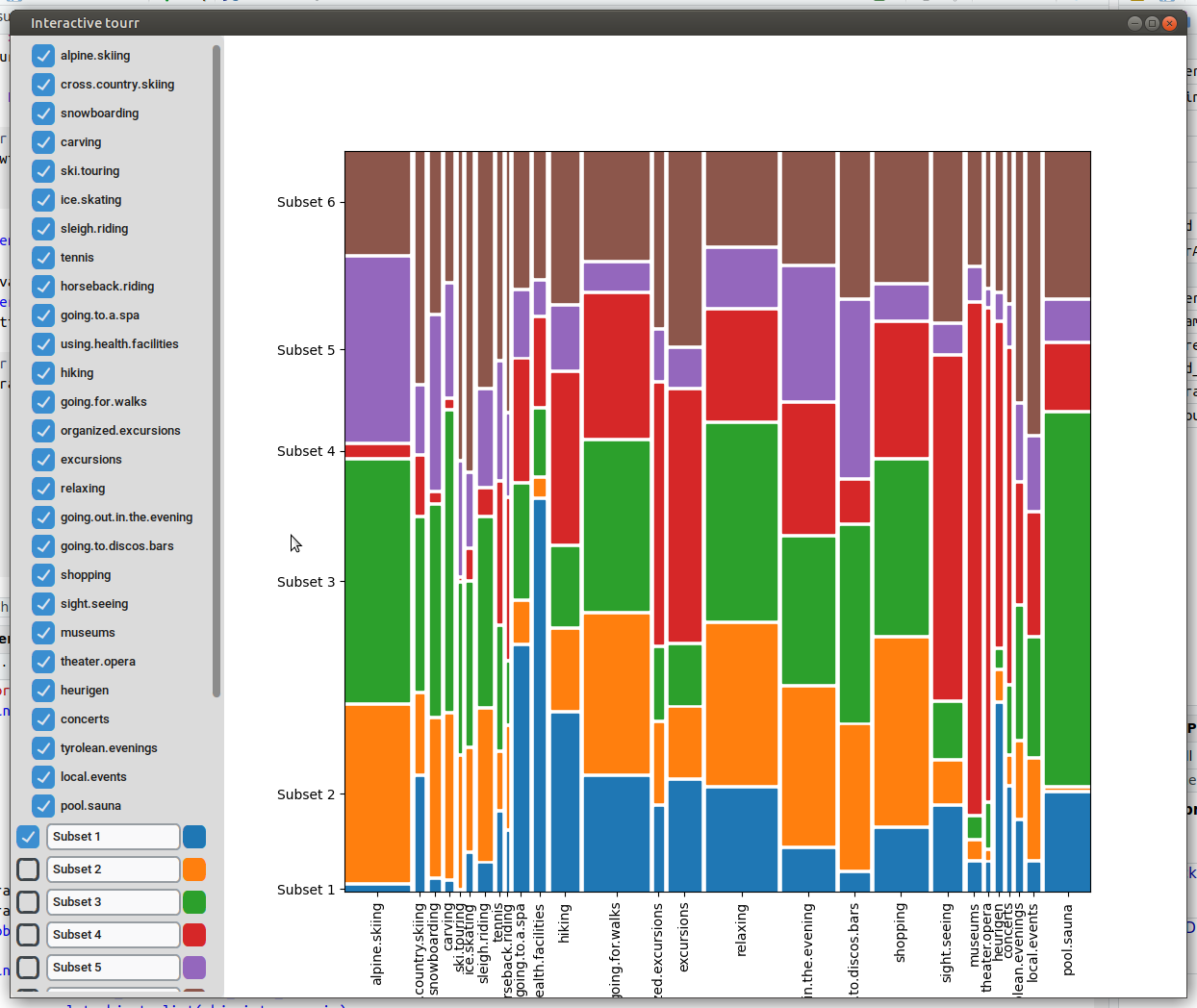
Mosaic
To display a mosaic plot, one has to provide whether the
subgroups/clusters should be on the x or y axis, either with
"subgroups_on_y" or "subgroups_on_x".
Example plot object
obj_winter_mosaic <- list(type="mosaic",   # type of display
                  obj=c("subgroups_on_y")) # whether subgroups x or y axis
Interactivity
Currently there is no way of directly interacting with the mosaic plot.
 {width=100%}
Heatmap
To display a heatmap, the metric to be calculated and plotted has to be
selected. One can choose between "Total fraction", "Intra cluster
fraction" and "Intra feature fraction".
Consider the matrix
[
C = \left[ \begin{array}{cccc} c_{11} & c_{12} & \dots & c_{1p} \
c_{21} & c_{22} & \dots & c_{2p} \
\vdots & \vdots & \ddots & \vdots \
c_{k1} & c_{k2} & \dots & c_{kp}
\end{array} \right]
]
where $c_{ij}, i=1, ..., k$ (number of clusters); $j=1, ..., p$ (number of
features) are a summary of each feature in each cluster. In case of binary
data $c_{ij}$ are the positive counts of the cluster/feature combination.
Then the total fraction is calculated by $f_{ij}^{o} = \frac{c_{ij}}{n}$
the intra cluster fraction by $f_{ij}^{c} = \frac{c_{ij}}{n_{i}}$ and
the intra feature fraction by $f_{ij}^{f} = \frac{c_{ij}}{n_{j}}$,
where $n_i, n_j$ are the row and column totals.
Example plot object
obj_winter_heatmap <- list(type="heatmap",          # type of display
                           obj=c("Total fraction")) # initial metric
Interactivity
- Metric selection: The currently displayed metric can be changed by using the
dropdown menu within the frame on the left. The details on the metrics can be
found above.
 {width=100%}
Categorical cluster interface
To display a categorical cluster interface, the metric to be calculated
and plotted has to be selected. One can choose between "Total fraction",
"Intra cluster fraction" and "Intra feature fraction". For details see "Heatmap"
Example plot object
obj_winter_cat_clust <- list(type="cat_clust_interface", # type of display
                             obj=c("Total fraction"))    # initial metric
Interactivity
- Metric selection: The currently displayed metric can be changed by using the
dropdown menu within the frame on the left. The details on the metrics can be
found above.
 {width=100%}
Generating the displays
The various plot objects can the be displayed with the
interactive_tour
function.
# interactive_tour call of flea dataset. Insert plot objects of your liking.
if (interactive()){
interactive_tour(data=flea,
                 feature_names=feature_names_flea,
                 plot_objects=list(obj_flea_2d_tour),
                 half_range=half_range_flea,
                 n_plot_cols=2,
                 preselection=clusters_flea,
                 n_subsets=3,
                 preselection_names=flea_subspecies,
                 display_size=5)
}
# interactive_tour call of winterActiv dataset. Insert plot objects of your liking.
if (interactive()){
interactive_tour(data=winterActiv,
                 feature_names=feature_names_winter,
                 plot_objects=list(obj_winter_cat_clust),
                 half_range=3,
                 n_plot_cols=2,
                 preselection=clusters_winter,
                 n_subsets=10,
                 display_size=5)
}
Try the lionfish package in your browser
Any scripts or data that you put into this service are public.
lionfish documentation built on April 4, 2025, 2:19 a.m.
R Package Documentation
Browse R Packages
We want your feedback!
Note that we can't provide technical support on individual packages. You should contact the package authors for that.
knitr::opts_chunk$set( collapse = TRUE, comment = "#>" )
Overview
The lionfish package offers multiple different types of display elements. These have to be provided to the interactive_tour function that launches the GUI. Each plot object is a list containing a type and an object. The type specifies, which kind of display should be generated. The object provides additional information required to construct the display. The plot objects then have to be stored in a list that can be given to the interactive_tour function. The currently supported displays are:
- 1d tour
- 2d tour
- scatterplot
- histogram
- mosaic plot
- heatmap
- categorical cluster interface
Examples for all displays can be found below.
Setup
# Load required packages library(tourr) library(lionfish) if (requireNamespace("flexclust")) {library(flexclust)}
# Initialize python backend if (check_venv()){ init_env(env_name = "r-lionfish", virtual_env = "virtual_env") } else if (check_conda_env()){ init_env(env_name = "r-lionfish", virtual_env = "anaconda") }
Dataset 1 - Flea data
# Load dataset data("flea") # Prepare objects for later us clusters_flea <- as.numeric(flea$species) flea_subspecies <- unique(flea$species) # Standardize data and calculate half_range flea <- apply(flea[,1:6], 2, function(x) (x-mean(x))/sd(x)) feature_names_flea <- colnames(flea) half_range_flea <- max(sqrt(rowSums(flea^2)))
Dataset 2 - Winter activities data
if (requireNamespace("flexclust")) { # Load dataset and set seed data("winterActiv") set.seed(42) # Perform kmeans clustering clusters_winter <- stepcclust(winterActiv, k=6, nrep=20) clusters_winter <- clusters_winter@cluster # Get the names of our features feature_names_winter <- colnames(winterActiv) }
Currently supported display types
One dimensional tour
To display one dimensional tours, they first have to be generated and saved using the save_history function of the tourr package. For more information on the available types of tours please visit tour path construction.
Example plot object
guided_tour_flea_1d <- save_history(flea, tour_path=guided_tour(holes(),1)) obj_flea_1d_tour <- list(type="1d_tour", # type of display obj=guided_tour_flea_1d) # 1d tour history
Interactivity
- Changing frames of tour: The frames of the current tour can be changed by pressing the left arrow-key for the last frame and the right arrow-key for the next frame. The current frame is displayed in the frame on the left.
- Projection manipulation: the projection can be manipulated clicking on one of the arrowheads with the right mouse-button and dragging it.
- Subselection: The datapoins within each subset can be changed by clicking on one of the bars of the histogram. The datapoints within the bar are then moved to the subset currently selected on the left.
{width=100%}
Two dimensional tour
To display two dimensional tours, they first have to be generated and saved using the save_history function of the tourr package. For more information on the available types of tours please visit tour path construction.
Example plot object
grand_tour_flea_2d <- save_history(flea, tour_path = grand_tour(d=2)) obj_flea_2d_tour <- list(type="2d_tour", # type of display obj=grand_tour_flea_2d) # 2d tour history
Interactivity
- Changing frames of tour: The frames of the current tour can be changed by pressing the left arrow-key for the last frame and the right arrow-key for the next frame. The current frame is displayed in the frame on the left.
- Projection manipulation: the projection can be manipulated clicking on one of the arrowheads with the right mouse-button and dragging it.
- Subselection: The datapoins within each subset can be changed by pressing the left mouse-button and drawing a lasso around the datapoints to be selected. The datapoints within the lasso are then moved to the subset currently selected on the left.
{width=100%}
Scatterplot
To display a scatter plot, the features to be displayed on the x and y axis have to be provided in form of a two dimensional vector.
Example plot object
obj_flea_scatter <- list(type="scatter", # type of display obj=c("tars1", "tars2")) # x and y axis of plot
Interactivity
- Subselection: The datapoins within each subset can be changed by pressing the left mouse-button and drawing a lasso around the datapoints to be selected. The datapoints within the lasso are then moved to the subset currently selected on the left.
{width=100%}
Histogram
To display a histogram, the feature to be displayed on the x axis has to be provided in form of a two dimensional vector.
Example plot object
obj_flea_histogram <- list(type="hist", # type of display obj="head") # x axis of histogram
Interactivity
- Subselection: The datapoins within each subset can be changed by clicking on one of the bars of the histogram. The datapoints within the bar are then moved to the subset currently selected on the left.
{width=100%}
Mosaic
To display a mosaic plot, one has to provide whether the subgroups/clusters should be on the x or y axis, either with "subgroups_on_y" or "subgroups_on_x".
Example plot object
obj_winter_mosaic <- list(type="mosaic", # type of display obj=c("subgroups_on_y")) # whether subgroups x or y axis
Interactivity
Currently there is no way of directly interacting with the mosaic plot.
{width=100%}
Heatmap
To display a heatmap, the metric to be calculated and plotted has to be selected. One can choose between "Total fraction", "Intra cluster fraction" and "Intra feature fraction".
Consider the matrix [ C = \left[ \begin{array}{cccc} c_{11} & c_{12} & \dots & c_{1p} \ c_{21} & c_{22} & \dots & c_{2p} \ \vdots & \vdots & \ddots & \vdots \ c_{k1} & c_{k2} & \dots & c_{kp} \end{array} \right] ]
where $c_{ij}, i=1, ..., k$ (number of clusters); $j=1, ..., p$ (number of features) are a summary of each feature in each cluster. In case of binary data $c_{ij}$ are the positive counts of the cluster/feature combination.
Then the total fraction is calculated by $f_{ij}^{o} = \frac{c_{ij}}{n}$
the intra cluster fraction by $f_{ij}^{c} = \frac{c_{ij}}{n_{i}}$ and
the intra feature fraction by $f_{ij}^{f} = \frac{c_{ij}}{n_{j}}$,
where $n_i, n_j$ are the row and column totals.
Example plot object
obj_winter_heatmap <- list(type="heatmap", # type of display obj=c("Total fraction")) # initial metric
Interactivity
- Metric selection: The currently displayed metric can be changed by using the dropdown menu within the frame on the left. The details on the metrics can be found above.
{width=100%}
Categorical cluster interface
To display a categorical cluster interface, the metric to be calculated and plotted has to be selected. One can choose between "Total fraction", "Intra cluster fraction" and "Intra feature fraction". For details see "Heatmap"
Example plot object
obj_winter_cat_clust <- list(type="cat_clust_interface", # type of display obj=c("Total fraction")) # initial metric
Interactivity
- Metric selection: The currently displayed metric can be changed by using the dropdown menu within the frame on the left. The details on the metrics can be found above.
{width=100%}
Generating the displays
The various plot objects can the be displayed with the interactive_tour function.
# interactive_tour call of flea dataset. Insert plot objects of your liking. if (interactive()){ interactive_tour(data=flea, feature_names=feature_names_flea, plot_objects=list(obj_flea_2d_tour), half_range=half_range_flea, n_plot_cols=2, preselection=clusters_flea, n_subsets=3, preselection_names=flea_subspecies, display_size=5) }
# interactive_tour call of winterActiv dataset. Insert plot objects of your liking. if (interactive()){ interactive_tour(data=winterActiv, feature_names=feature_names_winter, plot_objects=list(obj_winter_cat_clust), half_range=3, n_plot_cols=2, preselection=clusters_winter, n_subsets=10, display_size=5) }
Try the lionfish package in your browser
Any scripts or data that you put into this service are public.
R Package Documentation
Browse R Packages
We want your feedback!
Note that we can't provide technical support on individual packages. You should contact the package authors for that.
Embedding an R snippet on your website
Add the following code to your website.
For more information on customizing the embed code, read Embedding Snippets.