Stability Measures
In metasnf: Meta Clustering with Similarity Network Fusion

knitr::opts_chunk$set(
    collapse = TRUE,
    comment = "#>"
)

options(crayon.enabled = FALSE, cli.num_colors = 0)

Download a copy of the vignette to follow along here: stability_measures.Rmd

In this vignette, we will highlight the main stability measure options in the metasnf package.

Data set-up

library(metasnf)

my_dl <- data_list(
    list(cort_t, "cortical_thickness", "neuroimaging", "continuous"),
    list(cort_sa, "cortical_area", "neuroimaging", "continuous"),
    list(subc_v, "subcortical_volume", "neuroimaging", "continuous"),
    list(income, "household_income", "demographics", "continuous"),
    list(pubertal, "pubertal_status", "demographics", "continuous"),
    uid = "unique_id"
)

set.seed(42)
sc <- snf_config(
    my_dl,
    n_solutions = 4,
    max_k = 40
)

sol_df <- batch_snf(my_dl, sc)

To begin start calculating resampling-based stability measures, we'll build subsamples of the data list using the subsample_dl function.

my_dl_subsamples <- subsample_dl(
    my_dl,
    n_subsamples = 50,
    subsample_fraction = 0.85
)

my_dl_subsamples contains a list of 50 subsamples of the full data list. Each variation only has a random 85% of the original observations. Once the subsamples of the data list have been created, a cluster solution must be

batch_subsample_results <- batch_snf_subsamples(
    my_dl_subsamples,
    sc,
    verbose = TRUE
)

By default, the function returns a one-element list: cluster_solutions, which is itself a list of cluster solution data frames corresponding to each of the provided data list subsamples. Setting the parameters return_sim_mats and return_solutions to TRUE will turn the result of the function to a three-element list containing the corresponding solutions data frames and final fused similarity matrices of those cluster solutions, should you require these objects for your own stability calculations.

The function subsample_pairwise_aris can then be used to calculate the ARIs between cluster solutions across the subsamples.

pairwise_aris <- subsample_pairwise_aris(
    batch_subsample_results,
    verbose = TRUE
)

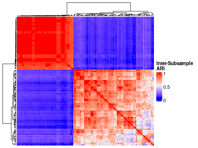
pairwise_aris is a list containing a summary data frame of the ARIs between subsamples for each row of the original settings data frame as well as another list of all the generated inter-subsample ARIs as a result of setting return_raw_aris to TRUE. The raw inter-subsample ARIs corresponding to a particualr settings data frame row can be visualized with a heatmap:

inter_ss_ari_hm <- ComplexHeatmap::Heatmap(
    pairwise_aris$"raw_aris"$"s1",
    heatmap_legend_param = list(
        color_bar = "continuous",
        title = "Inter-Subsample\nARI",
        at = c(0, 0.5, 1)
    ),
    show_column_names = FALSE,
    show_row_names = FALSE
)

save_heatmap(
    inter_ss_ari_hm,
    "vignettes/inter_ss_ari_hm.png",
    width = 400,
    height = 300,
    res = 70
)

{width=700px}

To calculate information about how often each pair of observations clustered together across the subsamples, we can use the calculate_coclustering function:

coclustering_results <- calculate_coclustering(
    batch_subsample_results,
    sol_df,
    verbose = TRUE
)

coclustering_results$"cocluster_summary"

The output of calculate_coclustering is a list containing the following components: - cocluster_dfs: A list of data frames, one per cluster solution, that shows the number of times that every pair of observations in the original cluster solution occurred in the same subsample, the number of times that every pair clustered together in a subsample, and the corresponding fraction of times that every pair clustered together in a subsample. - cocluster_ss_mats: The number of times every pair of observations occurred in the same subsample, formatted as a pairwise matrix. - cocluster_sc_mats: The number of times every pair of observations occurred in the same cluster, formatted as a pairwise matrix. - cocluster_cf_mats: The fraction of times every pair of observations occurred in the same cluster, formatted as a pairwise matrix. - cocluster_summary: Among pairs of observations that clustered together in the original cluster solution, the mean fraction those pairs remained clustered together across the subsample-derived solutions. This information is formatted as a data frame with one row per cluster solution.

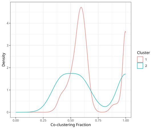
The cocluster_dfs component can be used to visualize co-clustering across subsamples as a density plot:

cocluster_dfs <- coclustering_results$"cocluster_dfs"

cocluster_density(cocluster_dfs[[1]])

{width=700px}

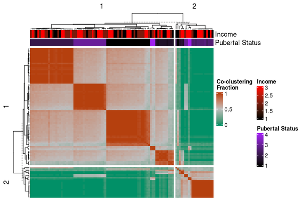
Or as a heatmap:

# Fraction of co-clustering between observations, grouped by original
# cluster membership
cocluster_heatmap(
    cocluster_dfs[[1]],
    dl = my_dl,
    top_hm = list(
        "Income" = "household_income",
        "Pubertal Status" = "pubertal_status"
    ),
    annotation_colours = list(
        "Pubertal Status" = colour_scale(
            c(1, 4),
            min_colour = "black",
            max_colour = "purple"
        ),
        "Income" = colour_scale(
            c(0, 4),
            min_colour = "black",
            max_colour = "red"
        )
    )
)