Nothing
README.md
In rmBayes: Performing Bayesian Inference for Repeated-Measures Designs
Bayesian Interval Estimation for Repeated-Measures Designs


For both the homoscedastic and heteroscedastic cases in one-way
within-subject (repeated-measures) designs, this Stan-based R package
provides multiple methods to construct the credible intervals for
condition means, with each method based on different sets of priors. The
emphasis is on the calculation of intervals that remove the
between-subjects variability that is a nuisance in within-subject
designs, as proposed in Loftus and Masson (1994), the Bayesian analog
proposed in Nathoo, Kilshaw, and Masson (2018), and the adaptation
presented in Heck (2019).
Installation
| Type | Source | Command |
|-------------|----------------------------------------------------|----------------------------------------------------|
| Release | CRAN | install.packages("rmBayes") |
| Development | GitHub | remotes::install_github("zhengxiaoUVic/rmBayes") |
R 4.0.1 or later is recommended. Prior to installing the package, you
need to configure your R installation to be able to compile C++ code.
Follow the link below for your respective operating system for more
instructions (version 2.26 or later; Stan Development Team, 2024):
- Mac - Configuring C++
Toolchain
- Windows - Configuring C++
Toolchain
- Linux - Configuring C++
Toolchain
Installation time of the source package is about 11 minutes (Stan models
need to be compiled). If you have R version 4.0.1 or later on Mac,
Windows, or Ubuntu, you can find the binary packages
HERE.
Or, directly install the binary package by preferably calling
install.packages("rmBayes", type = "binary")
Statistical Model
When the homogeneity of variance holds, a linear mixed-effects model
 for the mean response in a one-way within-subject design is


where
 represents the mean response for the
 th subject under the
 th level of the
experimental manipulation;
th level of the
experimental manipulation;
 is the overall
mean,
is the overall
mean,
 is the th level of the
experimental manipulation;
is the th level of the
experimental manipulation;
 ,
for the means model, is the
th condition mean;
,
for the means model, is the
th condition mean;
 are the
standardized subject-specific random effects;
are the
standardized subject-specific random effects;
 is the number of
levels;
is the number of
levels;  is the number
of subjects. The effects
is the number
of subjects. The effects
 and
are both
standardized relative to the standard deviation of the error
and
are both
standardized relative to the standard deviation of the error
 and become dimensionless (Rouder, Morey, Speckman, & Province, 2012).
Method 0
Nathoo et al. (2018) derived a Bayesian within-subject interval by
conditioning on maximum likelihood estimates of the subject-specific
random effects. An assumption articulated in Method 0 is the Jeffreys
prior for the condition means
 and
residual variance
and
residual variance
 ,
i.e.,
,
i.e.,
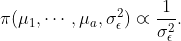
Method 0 constructs the highest-density interval (HDI) as
Note: The sample mean for the
th condition is
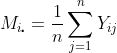 .
.
The sample mean for the
th subject is
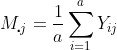 .
.
The overall mean is
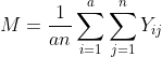 .
.
The within-group sum-of-squares (SS) is
 .
.
The interaction SS is
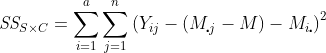 .
.
 refers to a
critical value for the
refers to a
critical value for the
 -distribution.
library(rmBayes)

str(recall.long)

rmHDI(recall.long, method = 0)
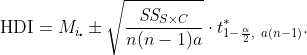
Methods 4-6
Heck (2019) proposed modifying the conditional within-subject Bayesian
interval to account for uncertainty and shrinkage in the estimated
random effects. He derived a modification by applying the HDI equation
in Method 0 for the within-subject Bayesian interval at each iteration
of a Markov chain Monte Carlo (MCMC) sampling algorithm and then taking
the average interval across posterior samples. Priors used in Method 4
are the Jeffreys prior for the condition means and residual variance, a
 -prior structure for
standardized subject-specific random effects (i.e.,
-prior structure for
standardized subject-specific random effects (i.e.,
 ),
and independent scaled inverse-chi-square priors with one degree of
freedom for the scale hyperparameters of the
-priors (i.e.,
),
and independent scaled inverse-chi-square priors with one degree of
freedom for the scale hyperparameters of the
-priors (i.e.,
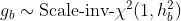 ).
).
Method 4 constructs the HDI as
![\text{HDI}=\mathbb{E}\left[\mu_{i}\pm\frac{\sigma_{\epsilon}}{\sqrt{n}}\cdot t_{1-\frac{\alpha}{2},\a(n-1)}^{*}\mid\text{Data}\right].](https://latex.codecogs.com/png.image?%5Ctext%7BHDI%7D%3D%5Cmathbb%7BE%7D%5Cleft%5B%5Cmu_%7Bi%7D%5Cpm%5Cfrac%7B%5Csigma_%7B%5Cepsilon%7D%7D%7B%5Csqrt%7Bn%7D%7D%5Ccdot%20t_%7B1-%5Cfrac%7B%5Calpha%7D%7B2%7D%2C%5C%20a%28n-1%29%7D%5E%7B%2A%7D%5Cmid%5Ctext%7BData%7D%5Cright%5D.)
rmHDI(recall.long, method = 4, seed = 277)
To assess the robustness of HDI results with respect to the choice of a
prior distribution for the standard deviation of the subject-specific
random effects in the within-subject case, two additional priors are
considered: uniform and half-Cauchy
( or
or
 )
for Methods 5 and 6, respectively.
)
for Methods 5 and 6, respectively.
rmHDI(recall.long, method = 5, seed = 277)
rmHDI(recall.long, method = 6, seed = 277)
Methods 1 (Default) and 2-3
Methods 0 and 4-6 arbitrarily assume improper uniform priors for the
condition means. In this work, Wei, Nathoo, and Masson (2023) expanded
the space of possible priors by appling the HDI equation in Method 0 to
derive the newly proposed intervals from MCMC sampling, but assuming
default -priors for
standardized treatment effects. In other words, Method 1 uses the
Jeffreys prior for the overall mean (rather than the condition means),
i.e.,
rmHDI(recall.long, seed = 277)
Similar to Methods 5 and 6, two additional priors are considered:
uniform and half-Cauchy
(
or
)
for Methods 2 and 3, respectively, for the standard deviation of the
subject-specific random effects in the within-subject case.
rmHDI(recall.long, method = 2, seed = 277)
rmHDI(recall.long, method = 3, seed = 277)
Standard HDI
MCMC sampling of condition means
can also
be used to obtain the standard HDI, which, unlike Methods 0-6, does not
remove the between-subjects variability that is not of interest in
within-subject designs. This method assumes the Jeffreys prior for the
overall mean and residual variance, a
-prior structure for
standardized treatment effects, and independent scaled
inverse-chi-square priors with one degree of freedom for the scale
hyperparameters of the
-priors.
rmHDI(recall.long, design = "between", seed = 277)
Random Versus Fixed Effects
When modeling fixed effects, Rouder et al. (2012, p. 363) proposed
default priors by projecting a set of
main effects into
 parameters such
that
parameters such
that
 ,
,
 ,
and
,
and
 ,
,
where
 is the identity matrix of size
,
is the identity matrix of size
,
 is the all-ones matrix of size
,
is the all-ones matrix of size
,
 is an
is an
 matrix of the
eigenvectors of unit length corresponding to the nonzero eigenvalues of
matrix of the
eigenvectors of unit length corresponding to the nonzero eigenvalues of
 ,
and
,
and
 is the row vector.
rmHDI(recall.long, treat = "fixed", seed = 277)
Heteroscedasticity
When the homogeneity of variance does not hold, the resulting HDI widths
for conditions are unequal. Two approaches are currently provided for
the heteroscedastic within-subject data: Implementing the approach
developed by Nathoo et al. (2018, p. 5);
rmHDI(recall.long, method = 0, var.equal = FALSE)
Or, implementing the heteroscedastic standard HDI method on the
subject-centering transformed data (subtracting from the original
response the corresponding subject mean minus the overall mean). If a
method option other than 0 or 1 is used with var.equal=FALSE, a
pooled estimate of variability will be used just as in the homoscedastic
case, and a warning message will be returned.
rmHDI(recall.long, var.equal = FALSE)
MCMC Diagnostics
Check the Rhat statistic and effective sample size of MCMC draws.
rmHDI(recall.long, seed = 277, diagnostics = TRUE)$diagnostics
References
Heck, D. W. (2019). Accounting for estimation uncertainty and shrinkage
in Bayesian within-subject intervals: A comment on Nathoo, Kilshaw, and
Masson (2018). Journal of Mathematical Psychology, 88, 27–31.
Loftus, G. R., & Masson, M. E. J. (1994). Using confidence intervals in
within-subject designs. Psychonomic Bulletin & Review, 1, 476–490.
Nathoo, F. S., Kilshaw, R. E., & Masson, M. E. J. (2018). A better
(Bayesian) interval estimate for within-subject designs. Journal of
Mathematical Psychology, 86, 1–9.
Rouder, J. N., Morey, R. D., Speckman, P. L., & Province, J. M. (2012).
Default Bayes factors for ANOVA designs. Journal of Mathematical
Psychology, 56, 356–374.
Stan Development Team (2024). RStan: the R interface to Stan. R package
version 2.32.5 https://mc-stan.org
Wei, Z., Nathoo, F. S., & Masson, M. E. J. (2023). Investigating the
relationship between the Bayes factor and the separation of credible
intervals. Psychonomic Bulletin & Review, 30, 1759–1781.
Try the rmBayes package in your browser
Any scripts or data that you put into this service are public.
rmBayes documentation built on May 29, 2024, 2:36 a.m.
R Package Documentation
Browse R Packages
We want your feedback!
Note that we can't provide technical support on individual packages. You should contact the package authors for that.
Bayesian Interval Estimation for Repeated-Measures Designs
![]()
![]()
For both the homoscedastic and heteroscedastic cases in one-way within-subject (repeated-measures) designs, this Stan-based R package provides multiple methods to construct the credible intervals for condition means, with each method based on different sets of priors. The emphasis is on the calculation of intervals that remove the between-subjects variability that is a nuisance in within-subject designs, as proposed in Loftus and Masson (1994), the Bayesian analog proposed in Nathoo, Kilshaw, and Masson (2018), and the adaptation presented in Heck (2019).
Installation
| Type | Source | Command |
|-------------|----------------------------------------------------|----------------------------------------------------|
| Release | CRAN | install.packages("rmBayes") |
| Development | GitHub | remotes::install_github("zhengxiaoUVic/rmBayes") |
R 4.0.1 or later is recommended. Prior to installing the package, you need to configure your R installation to be able to compile C++ code. Follow the link below for your respective operating system for more instructions (version 2.26 or later; Stan Development Team, 2024):
- Mac - Configuring C++ Toolchain
- Windows - Configuring C++ Toolchain
- Linux - Configuring C++ Toolchain
Installation time of the source package is about 11 minutes (Stan models need to be compiled). If you have R version 4.0.1 or later on Mac, Windows, or Ubuntu, you can find the binary packages HERE. Or, directly install the binary package by preferably calling
install.packages("rmBayes", type = "binary")
Statistical Model
When the homogeneity of variance holds, a linear mixed-effects model
for the mean response in a one-way within-subject design is
where
represents the mean response for the
th subject under the
th level of the
experimental manipulation;
is the overall
mean,
is the
th level of the
experimental manipulation;
,
for the means model, is the
th condition mean;
are the
standardized subject-specific random effects;
is the number of
levels;
is the number
of subjects. The effects
and
are both
standardized relative to the standard deviation of the error
and become dimensionless (Rouder, Morey, Speckman, & Province, 2012).
Method 0
Nathoo et al. (2018) derived a Bayesian within-subject interval by
conditioning on maximum likelihood estimates of the subject-specific
random effects. An assumption articulated in Method 0 is the Jeffreys
prior for the condition means
and
residual variance
,
i.e.,
Method 0 constructs the highest-density interval (HDI) as
Note: The sample mean for the
th condition is
.
The sample mean for the
th subject is
.
The overall mean is
.
The within-group sum-of-squares (SS) is
.
The interaction SS is
.
refers to a
critical value for the
-distribution.
library(rmBayes)
str(recall.long)
rmHDI(recall.long, method = 0)
Methods 4-6
Heck (2019) proposed modifying the conditional within-subject Bayesian
interval to account for uncertainty and shrinkage in the estimated
random effects. He derived a modification by applying the HDI equation
in Method 0 for the within-subject Bayesian interval at each iteration
of a Markov chain Monte Carlo (MCMC) sampling algorithm and then taking
the average interval across posterior samples. Priors used in Method 4
are the Jeffreys prior for the condition means and residual variance, a
-prior structure for
standardized subject-specific random effects (i.e.,
),
and independent scaled inverse-chi-square priors with one degree of
freedom for the scale hyperparameters of the
-priors (i.e.,
).
Method 4 constructs the HDI as
rmHDI(recall.long, method = 4, seed = 277)
To assess the robustness of HDI results with respect to the choice of a
prior distribution for the standard deviation of the subject-specific
random effects in the within-subject case, two additional priors are
considered: uniform and half-Cauchy
(
or
)
for Methods 5 and 6, respectively.
rmHDI(recall.long, method = 5, seed = 277)
rmHDI(recall.long, method = 6, seed = 277)
Methods 1 (Default) and 2-3
Methods 0 and 4-6 arbitrarily assume improper uniform priors for the
condition means. In this work, Wei, Nathoo, and Masson (2023) expanded
the space of possible priors by appling the HDI equation in Method 0 to
derive the newly proposed intervals from MCMC sampling, but assuming
default -priors for
standardized treatment effects. In other words, Method 1 uses the
Jeffreys prior for the overall mean (rather than the condition means),
i.e.,
rmHDI(recall.long, seed = 277)
Similar to Methods 5 and 6, two additional priors are considered:
uniform and half-Cauchy
(
or
)
for Methods 2 and 3, respectively, for the standard deviation of the
subject-specific random effects in the within-subject case.
rmHDI(recall.long, method = 2, seed = 277)
rmHDI(recall.long, method = 3, seed = 277)
Standard HDI
MCMC sampling of condition means
can also
be used to obtain the standard HDI, which, unlike Methods 0-6, does not
remove the between-subjects variability that is not of interest in
within-subject designs. This method assumes the Jeffreys prior for the
overall mean and residual variance, a
-prior structure for
standardized treatment effects, and independent scaled
inverse-chi-square priors with one degree of freedom for the scale
hyperparameters of the
-priors.
rmHDI(recall.long, design = "between", seed = 277)
Random Versus Fixed Effects
When modeling fixed effects, Rouder et al. (2012, p. 363) proposed
default priors by projecting a set of
main effects into
parameters such
that
,
,
and
,
where
is the identity matrix of size
,
is the all-ones matrix of size
,
is an
matrix of the
eigenvectors of unit length corresponding to the nonzero eigenvalues of
,
and
is the row vector.
rmHDI(recall.long, treat = "fixed", seed = 277)
Heteroscedasticity
When the homogeneity of variance does not hold, the resulting HDI widths for conditions are unequal. Two approaches are currently provided for the heteroscedastic within-subject data: Implementing the approach developed by Nathoo et al. (2018, p. 5);
rmHDI(recall.long, method = 0, var.equal = FALSE)
Or, implementing the heteroscedastic standard HDI method on the
subject-centering transformed data (subtracting from the original
response the corresponding subject mean minus the overall mean). If a
method option other than 0 or 1 is used with var.equal=FALSE, a
pooled estimate of variability will be used just as in the homoscedastic
case, and a warning message will be returned.
rmHDI(recall.long, var.equal = FALSE)
MCMC Diagnostics
Check the Rhat statistic and effective sample size of MCMC draws.
rmHDI(recall.long, seed = 277, diagnostics = TRUE)$diagnostics
References
Heck, D. W. (2019). Accounting for estimation uncertainty and shrinkage in Bayesian within-subject intervals: A comment on Nathoo, Kilshaw, and Masson (2018). Journal of Mathematical Psychology, 88, 27–31.
Loftus, G. R., & Masson, M. E. J. (1994). Using confidence intervals in within-subject designs. Psychonomic Bulletin & Review, 1, 476–490.
Nathoo, F. S., Kilshaw, R. E., & Masson, M. E. J. (2018). A better (Bayesian) interval estimate for within-subject designs. Journal of Mathematical Psychology, 86, 1–9.
Rouder, J. N., Morey, R. D., Speckman, P. L., & Province, J. M. (2012). Default Bayes factors for ANOVA designs. Journal of Mathematical Psychology, 56, 356–374.
Stan Development Team (2024). RStan: the R interface to Stan. R package version 2.32.5 https://mc-stan.org
Wei, Z., Nathoo, F. S., & Masson, M. E. J. (2023). Investigating the relationship between the Bayes factor and the separation of credible intervals. Psychonomic Bulletin & Review, 30, 1759–1781.
Try the rmBayes package in your browser
Any scripts or data that you put into this service are public.
R Package Documentation
Browse R Packages
We want your feedback!
Note that we can't provide technical support on individual packages. You should contact the package authors for that.
Embedding an R snippet on your website
Add the following code to your website.
For more information on customizing the embed code, read Embedding Snippets.