In CicciaLab/iSTOP: iSTOP - Induced STOP Experiment Design
knitr::opts_chunk$set(eval = F)
iSTOP
The iSTOP R package provides tools for designing induced stop mutations using CRISPR mediated base editing. It can perform a comprehensive search for iSTOP targetable codons present in a reference sequence (either in Fasta format, or from a BSgenome package). A tool for visualizing iSTOP targets across alternatively spliced isoforms is also included.
Installation
First, install R (~100 MB) and RStudio (~500 MB). Once installed, open RStudio and run the following commands in the R console to install all necessary R packages (~350 MB).
# Source the Biocoductor installation tool - installs and loads the
# BiocInstaller package which provides the biocLite function.
source("https://bioconductor.org/biocLite.R")

# Install the following required packages (dependencies will be included)
BiocInstaller::biocLite(c(
  # Packages from CRAN (cran.r-project.org)
  'tidyverse',
  'assertthat',
  'pbapply',
  'devtools',
  'fuzzyjoin',
  # Packages from Bioconductor (bioconductor.org)
  'BSgenome',
  'Biostrings',
  'GenomicRanges',
  'IRanges'))

# If all went well, install the iSTOP package hosted on GitHub
BiocInstaller::biocLite('CicciaLab/iSTOP')

# Now install a genome - e.g. for Human:
BSgenome::available.genomes() # To see what is conveniently available
BiocInstaller::biocLite('BSgenome.Hsapiens.UCSC.hg38') # ~850 MB

# And download CDS coordinates for your genome
# Be polite to UCSC - avoid repeated downloads!
CDS_Human <- iSTOP::CDS_Hsapiens_UCSC_hg38()
readr::write_csv(CDS_Human, '~/Desktop/CDS-Human.csv')
Quick usage examples
The following code demonstrates three common use cases, detecting iSTOP targets for (1) a single gene, (2) all genes that match a pattern, and (3) a set of transcript IDs. The workflow simply begins with CDS coordinates and a corresponding genomic sequence reference. We then:
- Choose the CDS coordinates for the transcripts we are interested in using
filter. Remove this step to search for all transcripts in your CDS coordinates table.
- Locate iSTOP codons (CAA, CAG, CGA, and TGG) in these transcripts using
locate_codons.
- Determine whether the codon has an available PAM using
locate_PAM.
- Annotate all targeted sites with enzymes that cut uniquely +/- 150 bases using
add_RFLP. Remove this step to reduce processing time.
library(tidyverse)
library(iSTOP)

# Read your previously saved CDS coordinates and prepare your genome
CDS_Human <- CDS_example()
Genome    <- BSgenome.Hsapiens.UCSC.hg38::Hsapiens

# (1) Detect iSTOP targets for a single gene
BRCA1 <-
  CDS_Human %>%
  filter(gene == 'BRCA1') %>%
  locate_codons(Genome) %>%
  locate_PAM(Genome) %>%
  add_RFLP(width = 150) %>%  # 150 is the maximum allowed
  add_RFLP(recognizes = 't') # Enzymes that cut if c edits to t

# (2) Detect iSTOP targets for genes that contain the string "BRCA"
BRCA <-
  CDS_Human %>%
  filter(grepl('BRCA', gene)) %>%
  locate_codons(Genome) %>%
  locate_PAM(Genome) %>%
  add_RFLP(width = 150)

# (3) Detect iSTOP targets for a set of transcript IDs
ATR <-
  CDS_Human %>%
  filter(tx %in% c('uc003eux.5', 'uc062ooq.1', 'uc062oor.1')) %>%
  locate_codons(Genome) %>%
  locate_PAM(Genome) %>%
  add_RFLP(width = 150)

View(ATR)
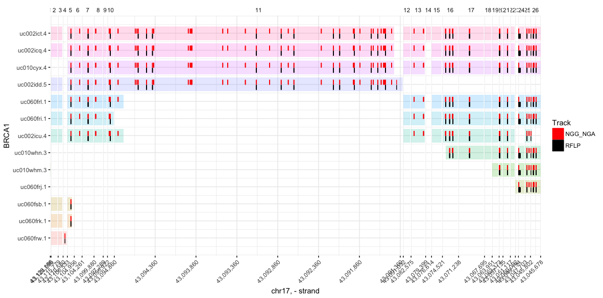
Visualize iSTOP coordinates
You can plot as many tracks as you like (though any more than 4 becomes difficult to read). Tracks can be named anything, and need only to be tables with at least two columns, (1) gene (gene names matching those in the CDS table), and (2) genome_coord (an integer indicating the genome coordinate to be marked in the track)
plot_spliced_isoforms(
  gene    = 'BRCA1',
  # Limit isoforms to those validated during iSTOP search
  coords  = filter(CDS_Human, tx %in% BRCA$tx),
  # Hex colors are also valid (e.g. #8bca9d)
  colors  = c('red', 'black'),
  # Name of track = table with columns `gene` and `genome_coord`
  NGG_NGA = filter(BRCA, has(sgNGG) | has(sgNGA)),   # `|` = or
  RFLP    = filter(BRCA, match_any  & has(RFLP_C_150)) # `&` = and
)
Detailed usage example
Load the following packages to make their contents available.
# Load packages to be used in this analysis
library(tidyverse)
library(iSTOP)
To locate iSTOP targets you will also need the following:
- CDS coordinates
- Genome sequence
CDS coordinates
This is an example table of CDS coordinates for S. cerevisiae RAD14.
| tx | gene | exon | chr | strand | start | end |
| :------ | :---- | :--- | :------ | :----- | :----- | :----- |
| YMR201C | RAD14 | 1 | chrXIII | - | 667018 | 667044 |
| YMR201C | RAD14 | 2 | chrXIII | - | 665845 | 666933 |
This gene has a single transcript "YMR201C" which is encoded on the "-" strand and has two exons (1 row for each exon). Note that, since this gene is encoded on the "-" strand, the first base in the CDS is located on chrXIII at position 667044, and the last base in the CDS is at position 665845. It is critial that exons are numbered with respect to CDS orientation. Chromosomes should be named to match the sequence names in your genome. Strand must be either "+", or "-".
The CDS function will generate a CDS table from annotation tables provided by the UCSC genome browser. Type ?CDS in the R console to view the documentation of this function. Note that the documentation for CDS lists several pre-defined functions to access complete CDS coordinates for a given species and genome assembly. The example below will download and construct a CDS coordinates table for the Human genome hg38 assembly. Note that only exons that contain coding sequence are retained, hence some transcripts not having coordinates for e.g. exon #1.
CDS_Human <- CDS_Hsapiens_UCSC_hg38()
Please be polite to UCSC by limiting the number of times you download their annotation files. I recommend saving the CDS coordinates locally by writing them to a CSV file. For example:
# You probably should pick a different location than the desktop...
CDS_Human %>% write_csv('~/Desktop/CDS-Hsapiens.csv')

# Then anytime you want to look up iSTOP targets, begin by reading this file
CDS_Human <- read_csv('~/Desktop/CDS-Hsapiens.csv')
Other pre-defined CDS functions include:
| Type | Species | CDS function |
| :---- | :---------------- | :------------------------------------- |
| Worm | C. elegans | CDS_Celegans_UCSC_ce11() |
| Fly | D. melanogaster | CDS_Dmelanogaster_UCSC_dm6() |
| Fish | D. rerio | CDS_Dreriio_UCSC_danRer10() |
| Human | H. sapiens | CDS_Hsapiens_UCSC_hg38() |
| Mouse | M. musculus | CDS_Mmusculus_UCSC_mm10() |
| Rat | R. norvegicus | CDS_Rnorvegicus_UCSC_rn6() |
| Yeast | S. cerevisiae | CDS_Scerevisiae_UCSC_sacCer3() |
| Plant | A. thaliana | CDS_Athaliana_BioMart_plantsmart28() |
Genome sequence
Using a BSgenome package
Pre-built genome sequence packages are provided by Bioconductor as "BSgenome" packages. To get a list of all available BSgenome packages you can run BSgenome::available.genomes(). For this example we will install the BSgenome package that corresponds to the Human hg38 assembly (as this matches the CDS coordinates we downloaded earlier).
# Note that the package only needs to be installed once.
BiocInstaller::biocLite('BSgenome.Hsapiens.UCSC.hg38')
Once installed we can access the genome object like so (Hint - type bsg then use RStudio's autocomplete to save some typing):
Genome_Human <- BSgenome.Hsapiens.UCSC.hg38::Hsapiens
Or, using fasta sequence files
Alternatively, you can construct a genome manually from a set of fasta files. Just make sure that the sequence names match those in the chr column of your CDS coordinates table and that the CDS coordinates are compatible with these sequences. This is not the recommended approach as sequence lookups are slower, but this is an option!
# Build custom genome of Human chromosomes X and Y
Genome_Human_XY <- Biostrings::readDNAStringSet(
  c('http://hgdownload.soe.ucsc.edu/goldenPath/hg38/chromosomes/chrX.fa.gz',
    'http://hgdownload.soe.ucsc.edu/goldenPath/hg38/chromosomes/chrY.fa.gz'))
Seach for iSTOP
# I will be limiting this analysis to chromosomes X and Y
Hooray <-
  CDS_Human %>%
  filter(chr %in% c('chrX', 'chrY')) %>%
  locate_codons(Genome_Human) %>%
  locate_PAM(Genome_Human)
# This analysis will be limited to PLCXD1 and uses the FASTA sequences
# Note that using FASTA sequences is MUCH slower than using a BSgenome
Hooray_XY <-
  CDS_Human %>%
  filter(gene == 'PLCXD1') %>%
  locate_codons(Genome_Human_XY) %>%
  locate_PAM(Genome_Human_XY)
Other features
locate_codons supports custom codon specificationlocate_PAM supports custom PAMs and custom spacingadd_RFLP supports custom enzymes sets
To access additional documentation for specific functions in the iSTOP package:
help(package = 'iSTOP')
Issues? Requests?
If you have a feature request or have identified an issue, please submit them on GitHub.
CicciaLab/iSTOP documentation built on May 9, 2021, 4:55 p.m.
R Package Documentation
Browse R Packages
We want your feedback!
Note that we can't provide technical support on individual packages. You should contact the package authors for that.
knitr::opts_chunk$set(eval = F)
iSTOP
The iSTOP R package provides tools for designing induced stop mutations using CRISPR mediated base editing. It can perform a comprehensive search for iSTOP targetable codons present in a reference sequence (either in Fasta format, or from a BSgenome package). A tool for visualizing iSTOP targets across alternatively spliced isoforms is also included.
Installation
First, install R (~100 MB) and RStudio (~500 MB). Once installed, open RStudio and run the following commands in the R console to install all necessary R packages (~350 MB).
# Source the Biocoductor installation tool - installs and loads the # BiocInstaller package which provides the biocLite function. source("https://bioconductor.org/biocLite.R") # Install the following required packages (dependencies will be included) BiocInstaller::biocLite(c( # Packages from CRAN (cran.r-project.org) 'tidyverse', 'assertthat', 'pbapply', 'devtools', 'fuzzyjoin', # Packages from Bioconductor (bioconductor.org) 'BSgenome', 'Biostrings', 'GenomicRanges', 'IRanges')) # If all went well, install the iSTOP package hosted on GitHub BiocInstaller::biocLite('CicciaLab/iSTOP') # Now install a genome - e.g. for Human: BSgenome::available.genomes() # To see what is conveniently available BiocInstaller::biocLite('BSgenome.Hsapiens.UCSC.hg38') # ~850 MB # And download CDS coordinates for your genome # Be polite to UCSC - avoid repeated downloads! CDS_Human <- iSTOP::CDS_Hsapiens_UCSC_hg38() readr::write_csv(CDS_Human, '~/Desktop/CDS-Human.csv')
Quick usage examples
The following code demonstrates three common use cases, detecting iSTOP targets for (1) a single gene, (2) all genes that match a pattern, and (3) a set of transcript IDs. The workflow simply begins with CDS coordinates and a corresponding genomic sequence reference. We then:
- Choose the CDS coordinates for the transcripts we are interested in using
filter. Remove this step to search for all transcripts in your CDS coordinates table. - Locate iSTOP codons (CAA, CAG, CGA, and TGG) in these transcripts using
locate_codons. - Determine whether the codon has an available PAM using
locate_PAM. - Annotate all targeted sites with enzymes that cut uniquely +/- 150 bases using
add_RFLP. Remove this step to reduce processing time.
library(tidyverse) library(iSTOP) # Read your previously saved CDS coordinates and prepare your genome CDS_Human <- CDS_example() Genome <- BSgenome.Hsapiens.UCSC.hg38::Hsapiens # (1) Detect iSTOP targets for a single gene BRCA1 <- CDS_Human %>% filter(gene == 'BRCA1') %>% locate_codons(Genome) %>% locate_PAM(Genome) %>% add_RFLP(width = 150) %>% # 150 is the maximum allowed add_RFLP(recognizes = 't') # Enzymes that cut if c edits to t # (2) Detect iSTOP targets for genes that contain the string "BRCA" BRCA <- CDS_Human %>% filter(grepl('BRCA', gene)) %>% locate_codons(Genome) %>% locate_PAM(Genome) %>% add_RFLP(width = 150) # (3) Detect iSTOP targets for a set of transcript IDs ATR <- CDS_Human %>% filter(tx %in% c('uc003eux.5', 'uc062ooq.1', 'uc062oor.1')) %>% locate_codons(Genome) %>% locate_PAM(Genome) %>% add_RFLP(width = 150) View(ATR)
Visualize iSTOP coordinates
You can plot as many tracks as you like (though any more than 4 becomes difficult to read). Tracks can be named anything, and need only to be tables with at least two columns, (1) gene (gene names matching those in the CDS table), and (2) genome_coord (an integer indicating the genome coordinate to be marked in the track)
plot_spliced_isoforms( gene = 'BRCA1', # Limit isoforms to those validated during iSTOP search coords = filter(CDS_Human, tx %in% BRCA$tx), # Hex colors are also valid (e.g. #8bca9d) colors = c('red', 'black'), # Name of track = table with columns `gene` and `genome_coord` NGG_NGA = filter(BRCA, has(sgNGG) | has(sgNGA)), # `|` = or RFLP = filter(BRCA, match_any & has(RFLP_C_150)) # `&` = and )
Detailed usage example
Load the following packages to make their contents available.
# Load packages to be used in this analysis library(tidyverse) library(iSTOP)
To locate iSTOP targets you will also need the following:
- CDS coordinates
- Genome sequence
CDS coordinates
This is an example table of CDS coordinates for S. cerevisiae RAD14.
| tx | gene | exon | chr | strand | start | end | | :------ | :---- | :--- | :------ | :----- | :----- | :----- | | YMR201C | RAD14 | 1 | chrXIII | - | 667018 | 667044 | | YMR201C | RAD14 | 2 | chrXIII | - | 665845 | 666933 |
This gene has a single transcript "YMR201C" which is encoded on the "-" strand and has two exons (1 row for each exon). Note that, since this gene is encoded on the "-" strand, the first base in the CDS is located on chrXIII at position 667044, and the last base in the CDS is at position 665845. It is critial that exons are numbered with respect to CDS orientation. Chromosomes should be named to match the sequence names in your genome. Strand must be either "+", or "-".
The CDS function will generate a CDS table from annotation tables provided by the UCSC genome browser. Type ?CDS in the R console to view the documentation of this function. Note that the documentation for CDS lists several pre-defined functions to access complete CDS coordinates for a given species and genome assembly. The example below will download and construct a CDS coordinates table for the Human genome hg38 assembly. Note that only exons that contain coding sequence are retained, hence some transcripts not having coordinates for e.g. exon #1.
CDS_Human <- CDS_Hsapiens_UCSC_hg38()
Please be polite to UCSC by limiting the number of times you download their annotation files. I recommend saving the CDS coordinates locally by writing them to a CSV file. For example:
# You probably should pick a different location than the desktop... CDS_Human %>% write_csv('~/Desktop/CDS-Hsapiens.csv') # Then anytime you want to look up iSTOP targets, begin by reading this file CDS_Human <- read_csv('~/Desktop/CDS-Hsapiens.csv')
Other pre-defined CDS functions include:
| Type | Species | CDS function |
| :---- | :---------------- | :------------------------------------- |
| Worm | C. elegans | CDS_Celegans_UCSC_ce11() |
| Fly | D. melanogaster | CDS_Dmelanogaster_UCSC_dm6() |
| Fish | D. rerio | CDS_Dreriio_UCSC_danRer10() |
| Human | H. sapiens | CDS_Hsapiens_UCSC_hg38() |
| Mouse | M. musculus | CDS_Mmusculus_UCSC_mm10() |
| Rat | R. norvegicus | CDS_Rnorvegicus_UCSC_rn6() |
| Yeast | S. cerevisiae | CDS_Scerevisiae_UCSC_sacCer3() |
| Plant | A. thaliana | CDS_Athaliana_BioMart_plantsmart28() |
Genome sequence
Using a BSgenome package
Pre-built genome sequence packages are provided by Bioconductor as "BSgenome" packages. To get a list of all available BSgenome packages you can run BSgenome::available.genomes(). For this example we will install the BSgenome package that corresponds to the Human hg38 assembly (as this matches the CDS coordinates we downloaded earlier).
# Note that the package only needs to be installed once. BiocInstaller::biocLite('BSgenome.Hsapiens.UCSC.hg38')
Once installed we can access the genome object like so (Hint - type bsg then use RStudio's autocomplete to save some typing):
Genome_Human <- BSgenome.Hsapiens.UCSC.hg38::Hsapiens
Or, using fasta sequence files
Alternatively, you can construct a genome manually from a set of fasta files. Just make sure that the sequence names match those in the chr column of your CDS coordinates table and that the CDS coordinates are compatible with these sequences. This is not the recommended approach as sequence lookups are slower, but this is an option!
# Build custom genome of Human chromosomes X and Y Genome_Human_XY <- Biostrings::readDNAStringSet( c('http://hgdownload.soe.ucsc.edu/goldenPath/hg38/chromosomes/chrX.fa.gz', 'http://hgdownload.soe.ucsc.edu/goldenPath/hg38/chromosomes/chrY.fa.gz'))
Seach for iSTOP
# I will be limiting this analysis to chromosomes X and Y Hooray <- CDS_Human %>% filter(chr %in% c('chrX', 'chrY')) %>% locate_codons(Genome_Human) %>% locate_PAM(Genome_Human)
# This analysis will be limited to PLCXD1 and uses the FASTA sequences # Note that using FASTA sequences is MUCH slower than using a BSgenome Hooray_XY <- CDS_Human %>% filter(gene == 'PLCXD1') %>% locate_codons(Genome_Human_XY) %>% locate_PAM(Genome_Human_XY)
Other features
locate_codonssupports custom codon specificationlocate_PAMsupports custom PAMs and custom spacingadd_RFLPsupports custom enzymes sets
To access additional documentation for specific functions in the iSTOP package:
help(package = 'iSTOP')
Issues? Requests?
If you have a feature request or have identified an issue, please submit them on GitHub.
R Package Documentation
Browse R Packages
We want your feedback!
Note that we can't provide technical support on individual packages. You should contact the package authors for that.
Embedding an R snippet on your website
Add the following code to your website.
For more information on customizing the embed code, read Embedding Snippets.