README.md

In FD155/ProjetR: Logistic Regression

GradDesc

This is a user manual of the R package GradDesc. The purpose of the GradDesc package is to make a binary logistic regression with the use of the stochastic gradient descent algorithm. It works on every dataset but the exploratory variables have to be quantitative and the target variable has to be binary. In this demonstration, we are going to use two different datasets : “breast_cancer” and "default_of_credit_card_clients" from UCI dataset to see how the algorithm behaves by exploiting the capacities of multicore processors.

Installing the package and access to the library

Once the package is installed, the library can be load using the standard commands from R.

install.packages("devtools")
library(devtools)

devtools::install_github("FD155/GradDesc")

library(GradDesc)

How to understand the expectations of the function parameters

You can just use the fonction help() to see all the documentation about your package. Then, you have acces to all the functions documentation.

help(package="GradDesc")

Short descriptions of datasets in the package

Breast Cancer :

This first dataset is about breast cancer diagnostic. Features are computed from a digitized image of a breast mass. The dataset contain 699 observations and 10 columns. The target variable is the class with two modalities : malignant cancer or begnin cancer.

Default of credit card clients :

The "default of credit card clients" data frame has 30 000 rows and 24 columns of data from customers default payments research. This research employed a binary variable, default payment (Yes = 1, No = 0), as the response variable.

Demonstration

Load your dataset

First, load your dataset on R like the example below. We begin with the shortest dataset, breast cancer. This dataset is included in the GradDesc package.

breast_cancer <- GradDesc::breast

If you want to import another dataset, use the code below.

library(readxl)
data <- read_excel("/Users/.../breast.xlsx")

Fit function

To use the GradDesc R package, the first function you have to call is the fit function which corresponds to the implementation of binary logistic regression with stochastic gradient descent. The possibility of exploiting the capacities of multicore processors is available for the batch mode of the gradient descent. To detect the number of cores you have access on your computer, use this code :

parallel::detectCores()

The gradient descent has three mode : the batch, mini-batch and online mode. Here, is an explanation of these mode in order to inform you which is the mode you want to apply.

Batch mode :

Batch gradient descent is a variation of the gradient descent algorithm that calculates the error for each example in the training dataset, but only updates the model after all training examples have been evaluated.

Mini-batch mode :

We use a batch of a fixed number of training examples which is less than the actual dataset and call it a mini-batch. The fixed number is call the batchsize and you can fix it in the fit function parameters.

Online mode :

In Stochastic Gradient Descent (SGD), we consider just one example at a time to take a single step.

Then, call the fit function and store the function call in an object variable. You have to informed the target variable and the explanatory variables in the formula parameter. The example below show you how to use the fit function.

LogisticRegression <- fit(formula=classe~.,data=data,coef=0.5,mode="batch",batch_size=0,learningrate=0.1,max_iter=100)

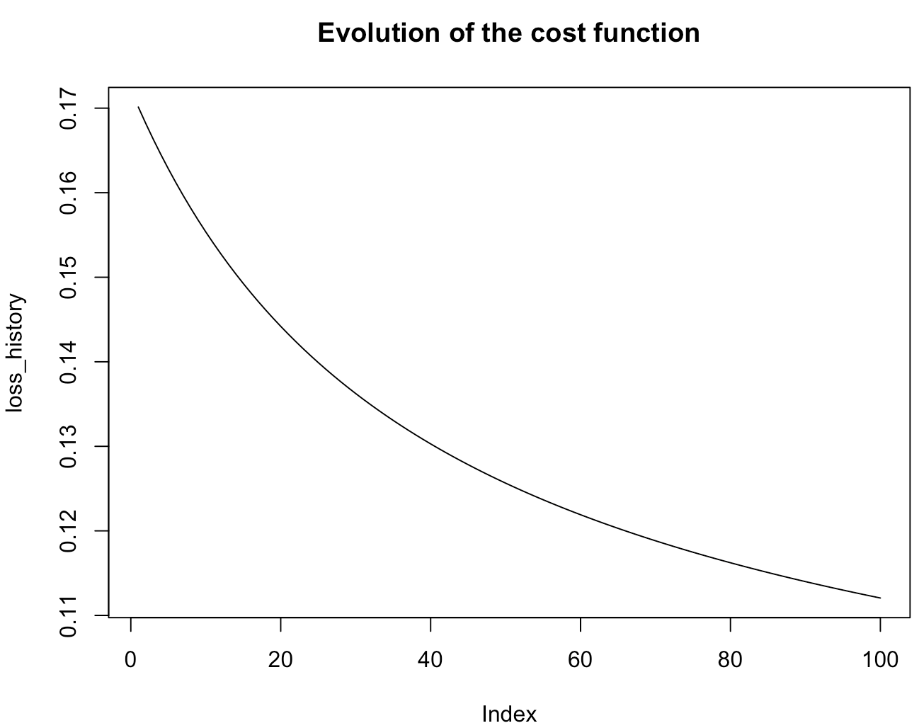
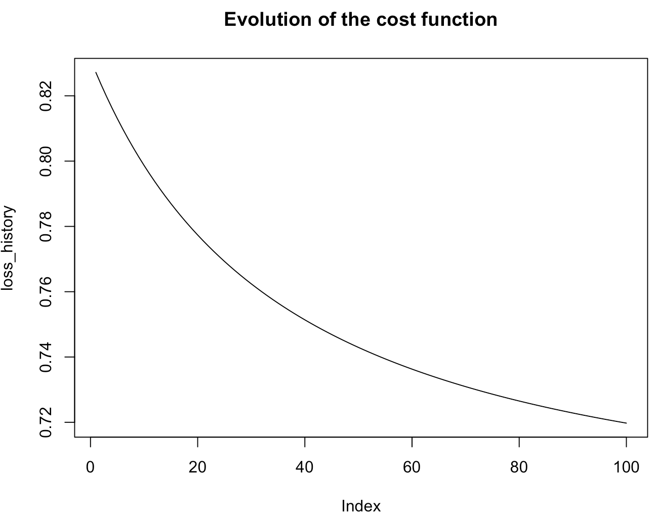
You must obtain a graphic like this one which show you the loss function according to the number of epochs. Here, we chose the mode "batch" of the gradient descent with a number of iteration fixed at 100.

To see the gradient descent, print or summarize it like this :

print(LogisticRegression)
summary(LogisticRegression)

The print call inform you which modality the algorithm takes as the positive modality. By default, it takes the modality that appears first in the dataset. This first call also show the number of epochs and the final coefficients of the gradient descent. You have access to the loss function at each iteration. The summary call also gives you the formula on which the descent gradient is based.

Now, let's see how the gradient descent behaves when using several ncores. Here, we chose to use 2 ncores on the fit function.

LogisticRegression <- fit(formula=classe~.,data=breast_cancer,coef=0.5,mode="batch",batch_size=10,learningrate=0.1,max_iter=100, ncores=2)

If you want to use more multicore processors, remember to see the number of cores on your computer with the code just above.

Now, you understand how to apply the fit function. Then, we use a bigger dataset to see the real utility of exploiting the capacities of multicore processors. That's why, we use the second dataset of the R package.

default_card <- GradDesc::DefaultOfCreditCards

We compare the batch mode with 1 ncore and then 3 ncores. To see the time of calculs, you can use "system.time".

print(system.time(LogisticRegression <- fit(formula=default~.,data=default_card,coef=0.5,mode="batch",batch_size=10,learningrate=0.1,max_iter=100, ncores=1)))

With one ncore, the time of the algorithm is about 23 seconds.

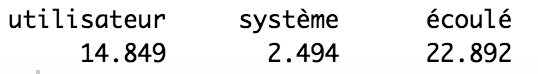
print(system.time(LogisticRegression <- fit(formula=default~.,data=default_card,coef=0.5,mode="batch",batch_size=10,learningrate=0.1,max_iter=100, ncores=3)))

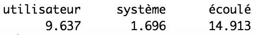
With three ncores, the time of the algorithm is now about 14 seconds. The result is clear, the gradient descent is achieved faster when using the capacity of multicore processors.

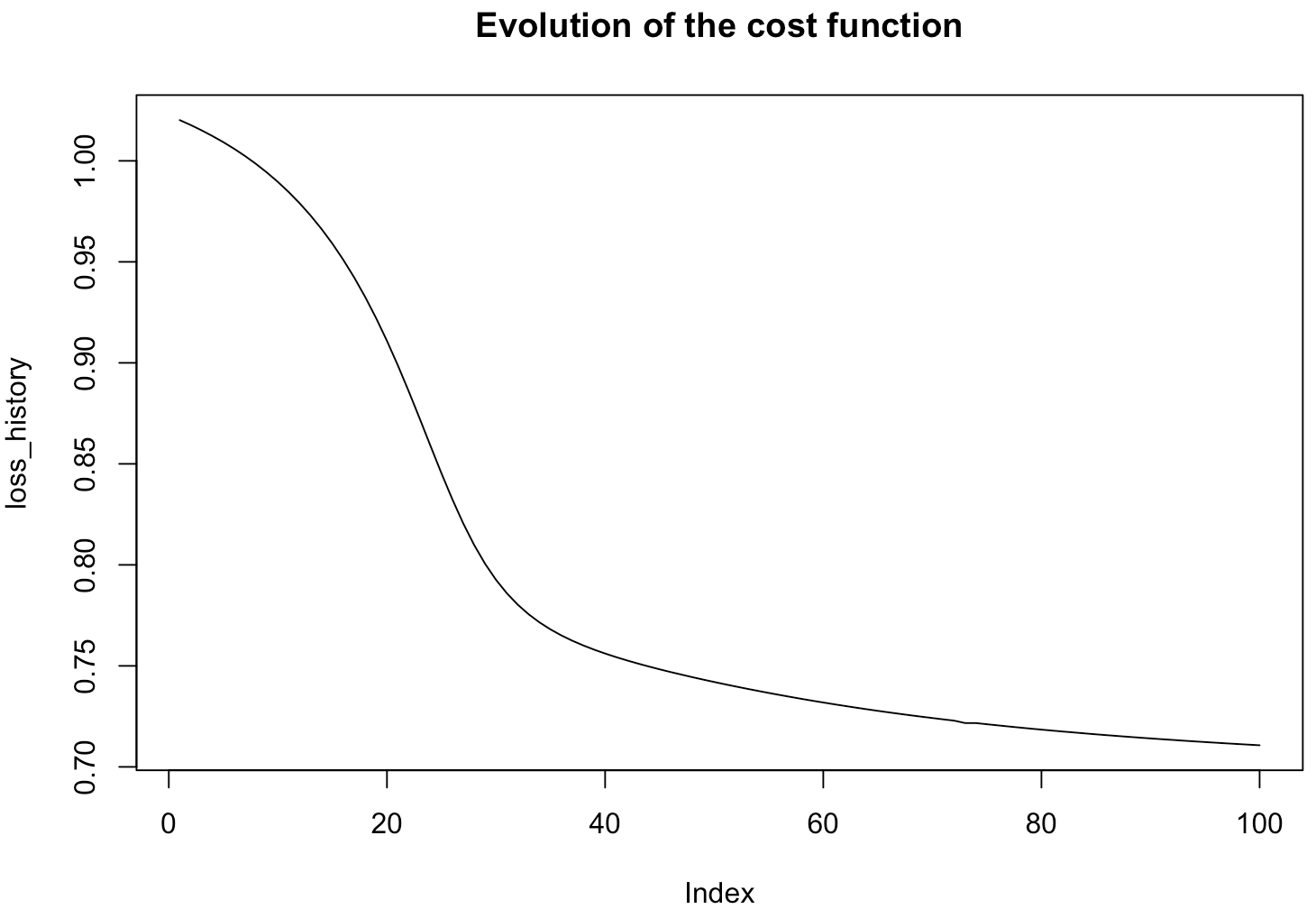
If you want to use the others mode of the gradient descent, here are some examples and output you can have. The exploitation of the capacities of multicore processors are not available on the mini-batch and online mode.

LogisticRegression <- fit(formula=default~.,data=default_card,coef=0.5,mode="mini-batch",batch_size=10,learningrate=0.1,max_iter=100, ncores=0)

LogisticRegression <- fit(formula=default~.,data=default_card,coef=0.5,mode="online",batch_size=1,learningrate=0.1,max_iter=100, ncores=0)

Predict function

The second function of the package is the predict function. Let's take our dataset "breast_cancer" and use the function like the example below.

data <- GradDesc::breast

First of all, we need to partition our dataset into learning and testing data. Use the package "caret" to do it.

install.packages("caret")
library(caret) #this package has the createDataPartition function

Then, we chose to take 75% for the learning part and 25% for the test part with the function "createDataPartition".

trainIndex <- createDataPartition(data$classe,p=0.75,list=FALSE)

Split the breast cancer data like this :

#splitting data into training/testing data using the trainIndex object
data_TRAIN <- data[trainIndex,] #training data (75% of data)
data_TEST <- data[-trainIndex,] #testing data (25% of data)
X_Test = data_TEST[,1:ncol(data)-1]
Y_Test = data_TEST[,ncol(data)]

We use the train data as input to the fit function.

print(system.time(LogisticRegression <- fit(formula=classe~.,data=data_TRAIN,coef=0.5,mode="batch",batch_size=1,learningrate=0.1,max_iter=100, ncores=0)))
print(LogisticRegression)
summary(LogisticRegression)

Let's take a look at the print and the summary function :

print(LogisticRegression)

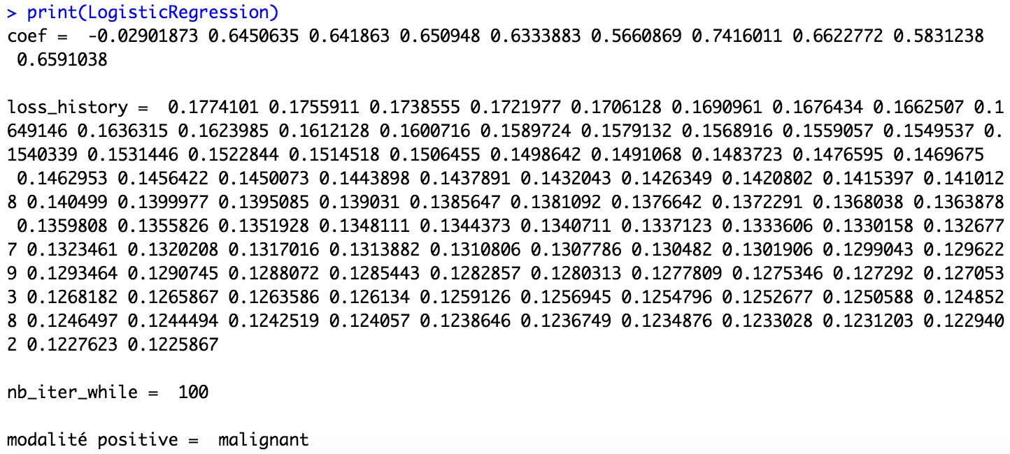
In this first function, you have access to the coefficients obtained thanks to the fit function. But more important, you have the positive modality which is take by the function. Here, it's the modality "malignant" which is the positive modality but sometimes, according to the partition of the dataset, it can be the other modality which is condider as the positive modality. So, take care about this information in the print function because the result of the confusion matrix depends on it.

summary(LogisticRegression)

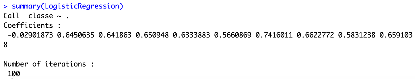
In this second function, you can see the formula of the model.

Call the predict function like this if you want to have the predict class for all of the observations.

pred <- predict(LogisticRegression,X_Test,type = "class")

According to the print function, we consider below that the positive modality is "malignant".

prediction <- as.matrix(ifelse(pred$pred==1, "malignant","begnin"))
Y_Test=as.matrix(Y_Test)

Show the confusion matrix like this, and see the result.

table(Y_Test,prediction)

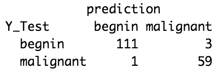
Here, we have only 4 false predictions. The prediction are pretty good. You can also see the proportion of the confusion matrix.

prop.table(table(Y_Test,prediction))

In order to get the percentage of correct predictions, we calculate the accuracy.

table <- table(Y_Test,prediction)
accuracy <- (table[1,1] + table[2,2]) / sum(table)
print(accuracy)

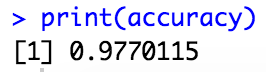
The accuracy is very close to 100%, signifying the strong performance of our model.

If you want to have the probability for each of the observations to belong to the class of the positive modality, chose the type "posterior" :

pred <- predict(LogisticRegression,X_Test,type = "posterior")

Let’s practice on your own dataset

Now that you have seen how the package works, it is up to you to use it on your own data. Remember to use the help() function to access to all the documentation.

Authors

Franck Doronzo, Candice Rajaonarivony, Gwladys Kerhoas

FD155/ProjetR documentation built on Dec. 17, 2021, 7:31 p.m.