In IMRpelagic/bifrost: Capelin assessment

knitr::opts_chunk$set(
  collapse = TRUE,
  cache = FALSE,
  comment = "#>",
  fig.path = "man/figures/README-",
  out.width = "80%",
  fig.height = 6,
  warning = FALSE
)

Bifrost package

Sondre Hølleland, Samuel Subbey

Institute of Marine Research, Norway.

Correspondance to: [e-mail], [e-mail]

Capelin assessment

This R package is a wrapper for doing capelin stock assessment.

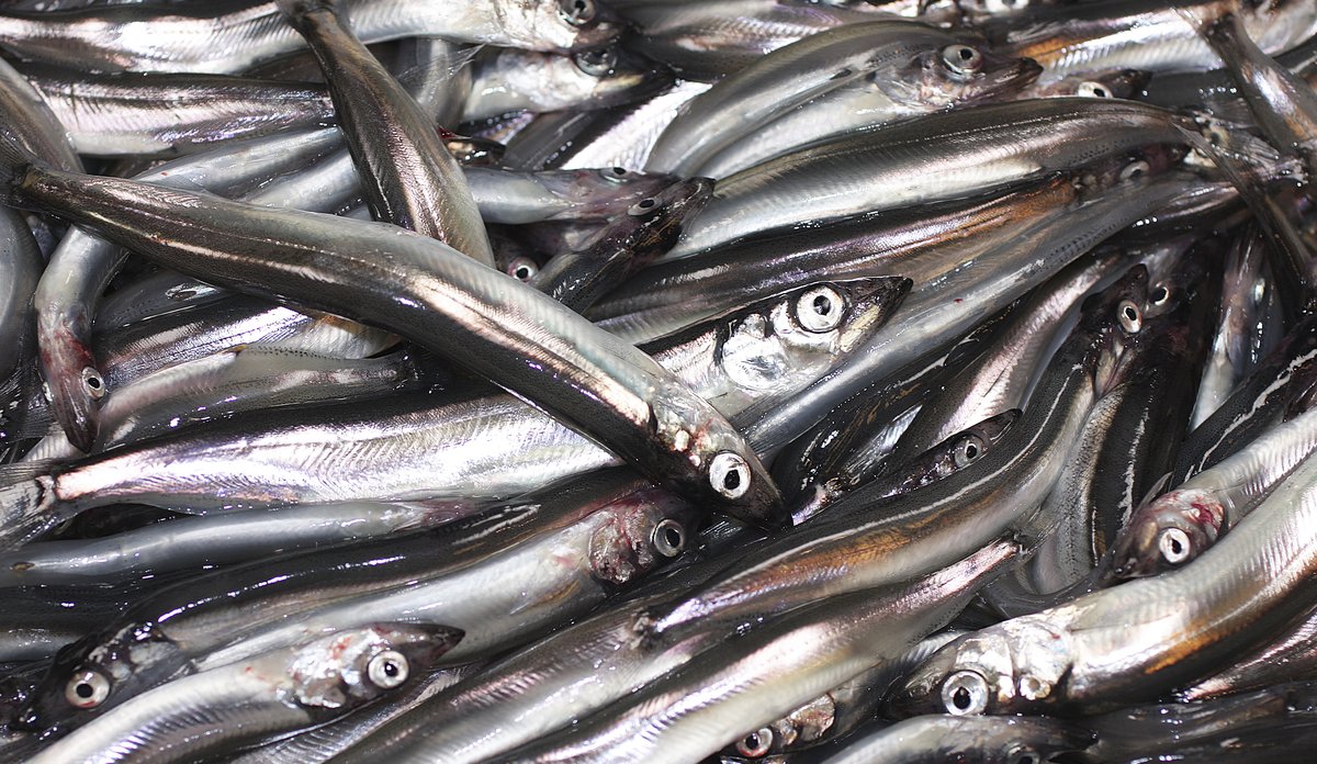
Capelin from the Barent Sea. Source: hi.no, Photographer: Jan de Lange / Institute of Marine Research

Documentation

A more detailed description can be found at https://imrpelagic.github.io/bifrostdocumentation/.

Install package

To install the package, run the following code:

library(devtools)
install_github("IMRpelagic/bifrost")

The package uses TMB (Template model builder).

For windows users, use the following code:

library(devtools)
install_github("IMRpelagic/bifrost", INSTALL_opts = "--NO-MULTIARCH")

Maturity

Here is an example to play with if you want to estimate maturity for capelin. In the package we have included a three datasets to help you get started with running the maturity estimation. First of all, you need to load the data:

library(bifrost)
# -- load the data --
data(cap) # capelin abundance table
data(catch) # capelin catch data
data(maturityInitialParameters) # initial parameters for 1972-2019
head(cap)
head(catch)
head(maturityInitialParameters)

Having the data loaded, we can set up the estimation procedure for the year 2003:

year <- 2010
#.. Create data list: ..
data.list <- createMaturityData(cap,
                                catch,
                                min_age = 2,
                                max_age = 3,
                                start_year =1972,
                                end_year = 2010)
# ..set up parameter list..
par.list <- createMaturityParameters(parameter = maturityInitialParameters,
                                    year = data.list$start_year, agegr = "2-3")
mFit <- estimateMaturity(data = data.list, parameters = par.list, silent =TRUE)
#.. Print estimates.. 
summary(mFit)

You can also run all years sequentially using the following function:

result <- runMaturityYearByYear(cap = cap, catch = catch, initPar = maturityInitialParameters,
                                min_age = 3, max_age = 4, plot = TRUE)
result$plot
plot(result)

Estimate consumption

data("consumptionData")
par.list <- list(
   logCmax   = log(1.2),
   logChalf  = log(1e2),
   logalpha  = log(2),
   logbeta   = log(2),
   logSigma  = log(1e3)
 )
 cFit <- estimateConsumption(data = consumptionData, parameters = par.list, silent =TRUE,
                             map  = list(logalpha = factor(NA),
                                         logbeta = factor(NA)))
 cFit
 summary(cFit)

Run simulations

We can run the simulation from October 1st to January 1st:

sim <- bifrost::captoolSim(mFit, nsim = 15000)
plot(sim)

We can also run the full simulation until April 1st:

catches <- 1000*colSums(catch[catch$year == 2010, c("spring01", "spring05", "spring04")])
fSim <- runFullSim(mFit, cFit, catches, nsim = 15000)
plot(fSim)

References

Put link to papers here.

In the development of this package, we have used

• TMB - the backbone of package
• TMBtools - helpful for makin an R package with using TMB

Licence

This project is licensed under the MIT licence - see LICENSE.md for details.

IMRpelagic/bifrost documentation built on Oct. 17, 2023, 7:11 a.m.