In ITSLeeds/pct: Propensity to Cycle Tool

knitr::opts_chunk$set(echo = TRUE)

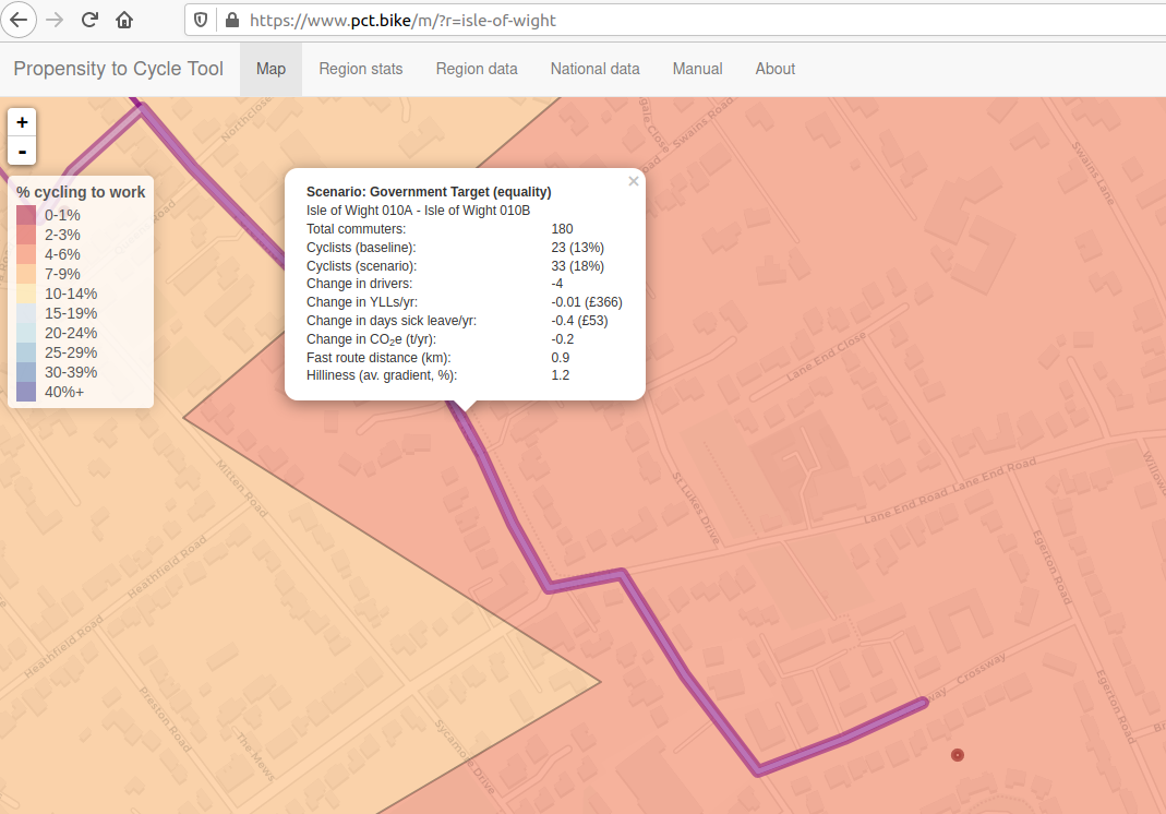
The desire line with the highest potential on the Isle of Wight looks like this:

The data hosted on the PCT website provides the same data with more precision:

library(dplyr)
l = pct::get_pct_lines("isle-of-wight")
l1 = l %>% 
  filter(bicycle == max(bicycle)) %>% 
  select(all, bicycle, rf_dist_km, rf_avslope_perc, govtarget_slc, dutch_slc) %>% 
  sf::st_drop_geometry()
l1
distance = l1$rf_dist_km

Based on that information we can calculate cycling uptake using the formulae from the manual as follows, first adjusting the hilliness level:

gradient = l1$rf_avslope_perc - 0.78

Government Target

The formula to calculate cycling uptake under the Government Target scenario is as follows:

Equation 1A:

logit (pcycle) = -4.018 + (-0.6369 * distance) + (1.988 * distance sqrt ) + (0.008775 distance sq ) + (-0.2555 * gradient) + (0.02006 * distancegradient) + (-0.1234 * distance sqrt *gradient) pcycle = exp ([logit (pcycle)]) / (1 + (exp([logit(pcycle)])

In code this can be written as:

logit_pcycle = -4.018 +
 (-0.6369 * distance) +
 (1.988 * sqrt(distance)) +
 (0.008775 * distance^2) +
 (-0.2555 * gradient) +
 (0.02006 * distance*gradient) +
 (-0.1234 * sqrt(distance) *gradient)
logit_pcycle
pcycle = exp(logit_pcycle) / (1 + exp(logit_pcycle))

Based on that, the scenario level of cycling would be:

pcycle 
pcycle * l1$all
pcycle * l1$all + l1$bicycle

Good news, this is the same as the govtarget_slc value in the data served by the PCT for that desire line (33 in both cases):

l1$govtarget_slc

Go Dutch

Cycling uptake under Go Dutch is calculated as follows.

Equation 1B:

logit(pcycle) = = -4.018 + (-0.6369 * distance) + (1.988 * distance sqrt ) + (0.008775 distance sq ) + (-0.2555 * gradient) + (0.02006 * distancegradient) + (-0.1234 * distance sqrt gradient) + (2.550 dutch) + (-0.08036 * dutch * distance)

Which can be simplified as:

logit_pcycle = -4.018 + 2.55 +
 ((-0.6369 - 0.08036) * distance) +
 (1.988 * sqrt(distance)) +
 (0.008775 * distance^2) +
 (-0.2555 * gradient) +
 (0.02006 * distance*gradient) +
 (-0.1234 * sqrt(distance) *gradient)
logit_pcycle
pcycle = exp(logit_pcycle) / (1 + exp(logit_pcycle))

Based on that, the scenario level of cycling would be:

pcycle 
pcycle * l1$all

However, the dutch_slc value in the data served by the PCT for that desire line is slightly higher:

l1$dutch_slc

Implementing the uptake model in a function

To ease reproducibility, the uptake formula can be represented in R functions:

remotes::install_github("itsleeds/pct")

library(pct)
uptake_pct_govtarget
uptake_pct_godutch_2020

We can check these reproduce the previous results as follows:

pcycle * l1$all
uptake_pct_godutch_2020(distance = l1$rf_dist_km, gradient = l1$rf_avslope_perc) *
  l1$all
uptake_pct_govtarget_2020(distance = l1$rf_dist_km, gradient = l1$rf_avslope_perc) *
  l1$all + l1$bicycle

Overall quality of fit

At the level of all OD pairs in the small region of the isle-of-wight, the correspondence between the results downloaded from the PCT website and the R implementation is as follows:

pcycle_package_govtarget = uptake_pct_govtarget(l$rf_dist_km, l$rf_avslope_perc)
pcycle_package_godutch = uptake_pct_godutch_2020(l$rf_dist_km, l$rf_avslope_perc)

govtarget_slc_package = pcycle_package_govtarget * l$all + l$bicycle
godutch_slc_package = pcycle_package_godutch * l$all 

plot(l$govtarget_slc, govtarget_slc_package)
plot(l$dutch_slc, godutch_slc_package)

cor(l$govtarget_slc, govtarget_slc_package)^2
cor(l$dutch_slc, godutch_slc_package)^2

cor(l$govtarget_sic, govtarget_slc_package)^2
cor(l$dutch_slc, godutch_slc_package + l$bicycle)^2

mean(l$govtarget_slc)
mean(govtarget_slc_package)

-(1 - mean(govtarget_slc_package) /
mean(l$govtarget_slc)) * 100

-(1 - mean(godutch_slc_package) /
mean(l$dutch_slc)) * 100

pcycle_gt_package = govtarget_slc_package / l$all
pcycle_gt_web = l$govtarget_slc / l$all

pcycle_gd_package = godutch_slc_package / l$all
pcycle_gd_web = l$dutch_slc / l$all

summary(100 * (pcycle_gt_package - pcycle_gt_web))
summary(100 * (pcycle_gd_package - pcycle_gd_web))