In ITSLeeds/slopes: Calculate Slopes of Roads, Rivers and Trajectories

# see slides manually uploaded online: https://slopes-slides.netlify.app/slides.html#1
# to run these slides locally:
xaringan::inf_mr("data-raw/slides.Rmd")

# From https://github.com/gadenbuie/xaringanExtra
xaringanExtra::use_xaringan_extra(c("tile_view", "animate_css", "tachyons"))

options(htmltools.dir.version = FALSE)
knitr::opts_chunk$set(
  fig.width=9, fig.height=3.5, fig.retina=3,
  out.width = "100%",
  # cache = TRUE,
  echo = TRUE,
  message = FALSE, 
  warning = FALSE,
  fig.show = TRUE,
  hiline = TRUE
)

library(xaringanthemer)
style_duo_accent(
  title_slide_background_color = "#FFFFFF",
  title_slide_background_size = "100%",
  title_slide_background_image = "https://user-images.githubusercontent.com/1825120/121391204-04c75c80-c946-11eb-8d46-ab5d8ada55c2.png",
  title_slide_background_position = "bottom",
  title_slide_text_color = "#080808",
  primary_color = "#080808",
  secondary_color = "#FF961C",
  inverse_header_color = "#FFFFFF"
)

background-image: url(https://camo.githubusercontent.com/30a3b814dd72aef5b51db635f2ab6e1b6b6c57b856d239822788967a4932d655/68747470733a2f2f7062732e7477696d672e636f6d2f6d656469612f45724a32647238574d414948774d6e3f666f726d61743d6a7067266e616d653d6c61726765) background-position: center background-size: 100%

--

Contents:

Why slopes?

--

Key functions

--

Future plans

--

---

Why we developed the slopes package

.left-column[

• Real world problems to solve involving slopes
• Existing tools were not up to the job
• Expensive and hard to reproduce findings (ESRI's 3D analyst)

• Hard to scale-up (online services)

• R programming challenge

• Support for route planning in active transportation

]

--

.right-column[

Real world problem: infrastructure prioritisation. Source: paper and www.pct.bike

]

???

• Rosa motivation

---

Applications

.left-column[

• Transport planning
• Active travel planning
• Logistics/route planning
• Emergency services
• River/flooding research
• Civil engineering

]

.right-column[

Image source: Goodchild (2020): Beyond Tobler’s Hiking Function

]

---

Installation and set-up

remotes::install_github("ropensci/slopes")

library(slopes)
library(tmap)
tmap_mode("view")

---

How the package works

Key functions:

1. slope_xyz(): calculates the slope associated with linestrings that have xyz coordinates
2. slope_raster(): Calculate slopes of linestrings based on local raster map
3. elevation_add(): Adds a third dimension to linestring coordinates
4. plot_slope(): Plots the slope profile associated with a linestring
5. See https://ropensci.github.io/slopes/reference/index.html for more

lisbon_route_3d_segments = stplanr::rnet_breakup_vertices(lisbon_route_3d)
lisbon_route_3d_segments$slope = slope_xyz(lisbon_route_3d_segments)
tm_shape(lisbon_route_3d_segments) +
  tm_lines(col = "slope", lwd = 3, palette = "viridis")

---

Package data

The key input datasets are:

--

.pull-left[

linestrings representing roads/rivers/other, and...

tm_shape(lisbon_road_network) + tm_lines()

]

--

.pull-right[

and digital elevations:

tm_shape(dem_lisbon_raster) + tm_raster(palette = "BrBG", alpha = 0.3)

]

---

Adding the Z dimension

lisbon_route

Dimension: XY

lisbon_route_slopes = elevation_add(routes = lisbon_route, dem = slopes::dem_lisbon_raster)

lisbon_route_slopes
## Simple feature collection with 1 feature and 3 fields
## Geometry type: LINESTRING
## Dimension:     XYZ

Dimension: XYZ

---

Plotting the Z dimension

.pull-left[

plot_slope(lisbon_route)

]

.pull-right[

plot_slope(lisbon_route_slopes)

]

---

Find slopes when you don't have a DEM

usethis::edit_r_environ()
# Type in (register on the mapbox website):
MAPBOX_API_KEY=xxxxx

library(stplanr)
origin = tmaptools::geocode_OSM("rail station zurich", as.sf = TRUE)
destination = tmaptools::geocode_OSM("eth zurich", as.sf = TRUE)
route = osrm::osrmRoute(src = origin, dst = destination, returnclass = "sf")
library(stplanr)
route = route(origin, destination, route_fun = cyclestreets::journey)
route_3d = elevation_add(route, dem = NULL)

route_3d$gradient_slopes = slope_xyz(route_3d) # todo: calculate slopes in elevation_add by default?

---

.pull-left[

library(tmap)
m = tm_shape(route_3d) + 
  tm_lines("gradient_slopes", lwd = 3,
           palette = "viridis")
tmap_mode("plot")
m
# Todo: add slope_map function with default palette?

]

.pull-right[

tmap_mode("view")
m

]

---

.pull-left[

Worked example

See vignette

Load packages

# Get linear features you want the gradients of
library(slopes)
library(dplyr)
library(sf)
# remotes::install_github("ITSLeeds/osmextract")
library(osmextract) # see UseR talk on osmextract package
library(tmap)
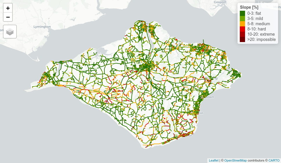
network = oe_get("Isle of Wight", vectortranslate_options = c("-where", "highway IS NOT NULL")) 

]

.pull-right[

u = "https://github.com/U-Shift/Declives-RedeViaria/releases/download/0.2/IsleOfWightNASA_clip.tif"
f = basename(u) # Get digital elevation data
download.file(url = u, destfile = f, mode = "wb")
dem = raster::raster(f)
library(raster)
plot(dem)
plot(sf::st_geometry(network), add = TRUE) #check if they overlay

]

---

Calculating slopes

sys_time = system.time({
  network$slope = slope_raster(network, dem)
})
sys_time
nrow(network)
nrow(network) / sys_time[3]

network$slope = network$slope * 100 # percentage
summary(network$slope) # check the values

---

Results

qtm(network, "slope") # with a few extra arguments...

See roadnetworkcycling vignette for details and here for interactive map: http://web.tecnico.ulisboa.pt/~rosamfelix/gis/declives/SlopesIoW.html

---

A smaller example using packaged data

routes = lisbon_road_network
dem = dem_lisbon_raster
routes$slope = slope_raster(routes, dem)
plot(dem)
plot(routes["slope"], add = TRUE)

---

Future plans

.pull-left[

• slope_get_dem() to get digital elevation model data
• Add other elevation sources using api keys (e.g Google, others)?
• Improve plot_slope() visualization
• Explore accuracy of data vs 'ground truth'
• Finish review, publish in JOSS and on CRAN
• See ropensci/slopes on github to get involved!

]

--

.pull-right[

]

???

invite people to help in github?

--

Blake Street, Sheffield. Source: thestar.co.uk

---

Where is the ground truth?

.pull-left[

• Comparison of gradients from the slopes packages and an online routing service

# route_3d$elevation_change
# route_3d$distances
plot(route_3d$gradient_smooth, route_3d$gradient_slopes)

]

.pull-right[

• How to get ground truth data? Quite hard!

]

---

Estimating slopes of bridges

knitr::include_graphics(c(
  "slope-edinburgh-bridge.png"
  # "slope-edinburgh-bridge2.png"
))

???

• RL

• My research into tools for prioritising cycling investment

• UK not very hilly but models fail slightly in hilly areas

---

knitr::include_graphics(c(
  # "slope-edinburgh-bridge.png",
  "slope-edinburgh-bridge2.png"
))

Thanks!

Slides created via the R packages:

xaringan
gadenbuie/xaringanthemer (And the Sharing Xaringan Slides blog post!)

The chakra comes from remark.js, knitr, and R Markdown.

ITSLeeds/slopes documentation built on Oct. 13, 2024, 3:54 a.m.