In JHuguenin/provoc: analyze data of VOC by PTR-ToF-MS Vocus

knitr::opts_chunk$set(
  collapse = TRUE,
  comment = "#>"
)
# knitr::opts_knit$set(root.dir = "C:/Users/huguenin/Documents/R/provoc")

provoc

Perform a Rapid Overview for Volatile Organic Compounds.

The provoc package has been developed to support PTR-ToF-MS users in their analyses. It has been designed for a quick import of data into R and visualization of the first results in a few minutes. It automatically detects peaks and provides a matrix for further analysis. Some chemometrics functions are proposed.

It is still a young and wild package that will appreciate feedback and new ideas for its development. Do not hesitate to contact the author to get or provide help.

For cite this package :

• Joris Huguenin, UMR 5175 CEFE, CNRS, University of Montpellier. provoc: analyze data of VOC by PTR-ToF-MS Vocus. DOI : 10.5281/zenodo.6642830.

Installation

The development version can be installed from GitHub using:

# install.packages("remotes")
remotes::install_github("jhuguenin/provoc")

The package requires the update of many dependencies:

• baseline(>= 1.3.0)
• dygraphs(>= 1.1.0)
• graphics(>= 4.0.0)
• grDevices(>= 4.0.0)
• Iso(>= 0.0-18.1)
• magrittr(>= 2.0.0)
• MALDIquant(>= 1.19.0)
• nnls(>= 1.4)
• rhdf5(>= 2.34.0)
• rmarkdown(>= 2.11.0)
• scales(>= 1.1.0)
• stats(>= 4.0.0)
• stringr(>= 1.4.0)
• viridis(>= 0.6.0)
• usethis(>= 2.1.0)
• utils(>= 4.0.0)
• xts(>= 0.12.0)

Description of function

Principals functions

• import.h5 for import you data. Easy.
• import.meta custom your analysis plans.
• dy.spectra & fx.spectra look at your dynamic or fixed spectra.
• kinetic.plot look the kinetic of your VOCs.
• mcr.voc perform a MCR analysis on your data.

Secondary functions

Manage your data

• if you can't import your files, look them with info.h5. After that, delete a corrupted spectra with delete.spectra.h5.
• peek your meta data with meta.ctrl and the peak alignment with peak.ctrl.
• manage the time of your data with re.calc.T.para or revert to original data by re.init.T.para.
• create a new file "meta_empty.csv" : empty.meta.

Find index or position

• ind.acq return index of spectra for each acquistion.
• ind.pk return index of peaks.
• det.c return the index more closed of a decimal number in the numeric vector.
• M.Z search all peak in accord to a mass number
• M.Z.max search the highest peak in accord to a mass number

Usage

library(provoc)

Importation

Before importing, all h5 files must be placed in a directory named h5. This directory must be placed in the working directory. The name of the h5 files placed in the directory may contain the date and time of recording in the form _yyymmdd_hhmmss. This information will be removed during import. e.g. 00_file_PTR_ToF_MS_20210901_093055.h5 will be renamed 00_file_PTR_ToF_MS by the import.

Each file is an acquisition with several spectra.

# working directory
wd <- "~/R/data_test/miscalenous" # without final "/"
setwd(wd) # If you you don't work by project.

# + wd/
# |  \- h5/
# |     \- 00_file_PTR_ToF_MS.h5
# |     \- 01_file_PTR_ToF_MS.h5
# |     \- 02_file_PTR_ToF_MS.h5

# import
sp <- import.h5(wd) # or just sp <- import.h5() if you work by project. 

The import.h5() function automatically creates a directory named "Figures", a csv file with the meta data "meta_empty.csv" and a list sp. This list contains :

• MS : a big matrix with all data.
• peaks : a short matrix with peak intensity.
• xMS : vector for the MS abscissa.
• names : folder names use in this meta set.
• wd : the working directory.
• acq : ID use in this meat seta.
• nbr_sp : the number of spectra for each acquisition.
• names_acq : names of spectra.
• Tinit : the original date (and time) of spectra.
• Trecalc : the recalculated time of spectra (for cumulated several acquisition).
• workflow : the list of each operation in the project.
• mt : the R meta data.
• meta : the Vocus meta data.

You can control part of the analysis with the "meta_empty.csv" file. It is in the form of a table with all the acquisitions imported in rows. The columns are :

• names : names of acquisiton.
• ID : identifier number.
• nbr_MS : number of spectra in this acquisition.
• start : the index where this acquisition begins.
• end : the index where this acquisition ends.
• used : TRUE/FALSE selects the acquisitions useful for the analysis.
• blank (ID) : (not available) subtract the blank.
• color : specifies a color.
• concentration : (not available) specifies a concentration.
• unit : (not available) and the unit of concentration.
• acq_T0 (ID) : the T0 ID of the sequence.
• delta_T (s) : It's possible to adjust the sequence by a shift time in second.
• grp1, grp2, ... : others free columns for analyzes. Names of columns can be changed.

You can prepare several meta files. By activating or not the acquisitions, it is possible to make different analyses. This allows you to do only one import (often long). You can rename the files meta_1, meta_2 or with more explicit names.

If the import is stopped because of a corrupted file, use info.h5() and delete.spectra.h5() to correct this file.

If your h5 files are differents, let me know and I can add an option for you.

Optimize the importation

If you want to improve the data import, there are three options to consider :

• First, a baseline correction step can be added with: baseline_correction = TRUE. When the instrument receives a large number of molecules with the same mass, the detector fluctuates slightly which leaves a visible trace on the spectrogram. This baseline correction is a time consuming but very effective step to improve the analysis.
• Then, the parameters for detecting and aligning the peaks can be adjusted according to the experiment. The package proposes some predefined parameters (see pk_param) but the user can modify these parameters (mainly the size of the width of the peak at half height "halfWindowSize" and the signal to noise ratio "SNR"). The quality of these parameters can be visualized thanks to the ctrl_peak argument.
• Finally, the argument skip = X allows not to import the first X spectra of each file. Typically, in a sequence with several channels, the first spectra will always be polluted by the previous channel. Not importing them saves RAM and computation time. It also allows to import longer sequences in one go.

Preparation

After the import, a csv file was created in the working directory. This file should look like this:

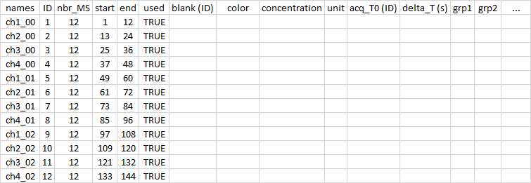
It is made to be easily opened and closed by excel in Windows10. If your default settings do not allow this facility, let me know and I can add an option for you.

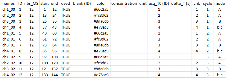
Once opened, you can edit the information inside to fill in different information such as the color or modality of your samples. Here, the example shows the first three cycles of a sequence with four samples, two with modality A, one with modality B and one blank. There are 12 spectra per sample.
With the column acq_T0, I indicate which acquisitions belong to each sample. This is useful for the "time" option when producing the graph.

sp <- import.meta("meta_1") # without '.csv'

Then, to refine my analysis, I decided to superimpose the T0 of each sample to facilitate the comparison. For this, I removed 300 (600 and 900) seconds because each sample is analyzed for 5 minutes. I also removed my sample 2 with the used column. Finally, I selected only the last 6 spectra (out of 12) by modifying the start column.

sp <- import.meta("meta_2")

To be able to switch from one graphical representation to another quickly, I created two files meta_1.csv and meta_2.csv that I import according to my needs.

All operations performed during the analysis are recorded. It is easy to save this trace. Afterwards, you can restart your workflow automatically (not available).

saveRDS(sp$workflow, "workflow.rds")
wf <- readRDS("workflow.rds")

After preparing the meta file, you should recalculate the time with re.calc.T.para() if you need to. The other function reinitialize the time.

sp <- re.calc.T.para(sp)
sp <- re.init.T.para(sp)

Be careful. By default, the "time" option uses a relative T0 from the first spectrum of each acquisition and the "date" option uses the actual date and time of each spectrum. Using the acq_T0 column with the "time" option allows different acquisitions to be sequenced using the T0 of the specified acquisition. Using the acq_T0 column with the "date" option allows you to overlap acquisitions on the T0 of the specified acquisition.

The delta_T column is used to add the specified time (in seconds) to the acquisition.

Make a plot

With the following three functions, it is really easy to make graphs to explore your data.

dy.spectra and fx.spectra allow you to make figures of the spectra, respectively dynamically and fixed. You have to fill sel_sp with a numerical vector indicating the numbers of the spectra to use (sp$Sacq). For fx.spectra, pkm and pkM are the min and max limits.

# a dynamic plot :
dy.spectra(sel_sp = sp$mt$meta[sp$acq,"end"], new_color = FALSE)
# a standart plot :
fx.spectra(sel_sp = sp$mt$meta[sp$acq,"end"], pkm = 137, pkM = 137, leg = "l")
fx.spectra(sel_sp = 1, pkm = 59, pkM = 150)

kinetic.plot plots the evolution of the peaks.

• M_num : Analyzed masses. M.Z(c(69, 205, 157)), M.Z.max(c(69, 205, 157)) or c(69.055, 205.158, 157.021).
• each_mass : make a plot for each masse or not. Logical TRUE or FALSE.
• group : the name of the meta column that categorizes the groups, or not. e.g. : "grp1" or FALSE.
• graph_type : choice "fx" for fixed plot (.tiff) or "dy" for dynamic plot (.html)
• Y_exp : y axe exponential or not. Logical TRUE or FALSE.
• time_format : x axe with a time ("time") or with a date ("date").

kinetic.plot(M_num = M.Z.max(c(59, 137)), each_mass = TRUE,
                         group = "grp1", graph_type = "dy",
                         Y_exp = FALSE, time_format = "date")

Make a MCR

After performing a univariate analysis, Provoc allows a multivariate analysis using the MCR algorithm. This technique is detailed in the article : Multivariate Curve Resolution (MCR). Solving the mixture analysis problem(2014). Anna de Juan, Joaquim Jaumot and Roma Tauler. https://doi.org/10.1039/C4AY00571F

Currently the constraints of the MCR are by default the same as those of the "alsace" package. They are consistent with an analysis of PTR-ToF-MS data. The function allows to set the number of components used for the RCM (ncMCR) and to specify a variable selection (pk_sel). You can also specify a column from the meta_xxx.csv file that you wish to use to group the spectra according to a modality.

Arguments - ncMCR : (integer) number of componant of MCR. - grp : a character string of the group 's column name. - pk_sel : a vector of selected peaks, or "all". - time_format : a charater string "date" or "time". - Li : the list with spectra (sp).

mcr.result <- mcr.voc(ncMCR = 3, grp = "modality", pk_sel = "all", 
                      time_format = "date", Li = sp)

Others functions

The package includes several small utility functions.
Three of them deserve a clear explanation because they allow you to find the index of peaks or spectra. ind.acq allows you to find the spectra related to an acquisition. For example, if you have taken a series of 60 acquisitions, each with 8 spectra, ind.acq allows you to locate the 8 spectra of the 42nd acquisition [ ind.acq(42) #329 330 331 332 333 334 335 336]. ind.pk works in the same way but on the position of the peaks. This function should not be confused with M.Z (or M.Z.max) which finds the peaks detected during the import.

And now ...

You have everything to work wit provoc. If you have specific needs, questions or remarks, you can contact me quickly at my email address (joris.name [at] cefe.cnrs.fr).

See you

JHuguenin/provoc documentation built on Jan. 29, 2024, 12:39 a.m.