In JuliaDiffEq/diffeqr: Solving Differential Equations (ODEs, SDEs, DDEs, DAEs)
knitr::opts_chunk$set(
  collapse = TRUE,
  comment = "#>"
)
1D Linear ODEs
Let's solve the linear ODE u'=1.01u. First setup the package:
de <- diffeqr::diffeq_setup()
Define the derivative function f(u,p,t).
f <- function(u,p,t) {
  return(1.01*u)
}
Then we give it an initial condition and a time span to solve over:
u0 <- 1/2
tspan <- c(0., 1.)
With those pieces we define the ODEProblem and solve the ODE:
prob = de$ODEProblem(f, u0, tspan)
sol = de$solve(prob)
This gives back a solution object for which sol$t are the time points
and sol$u are the values. We can treat the solution as a continuous object
in time via
and a high order interpolation will compute the value at t=0.2. We can check
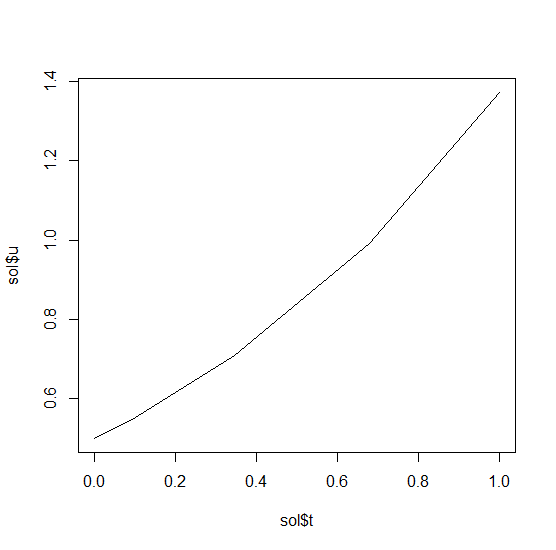
the solution by plotting it:
plot(sol$t,sol$u,"l")
Systems of ODEs
Now let's solve the Lorenz equations. In this case, our initial condition is a vector and our derivative functions
takes in the vector to return a vector (note: arbitrary dimensional arrays are allowed). We would define this as:
f <- function(u,p,t) {
  du1 = p[1]*(u[2]-u[1])
  du2 = u[1]*(p[2]-u[3]) - u[2]
  du3 = u[1]*u[2] - p[3]*u[3]
  return(c(du1,du2,du3))
}
Here we utilized the parameter array p. Thus we use diffeqr::ode.solve like before, but also pass in parameters this time:
u0 <- c(1.0,0.0,0.0)
tspan <- list(0.0,100.0)
p <- c(10.0,28.0,8/3)
prob <- de$ODEProblem(f, u0, tspan, p)
sol <- de$solve(prob)
The returned solution is like before except now sol$u is an array of arrays,
where sol$u[i] is the full system at time sol$t[i]. It can be convenient to
turn this into an R matrix through sapply:
mat <- sapply(sol$u,identity)
This has each row as a time series. t(mat) makes each column a time series.
It is sometimes convenient to turn the output into a data.frame which is done
via:
udf <- as.data.frame(t(mat))
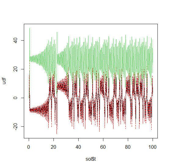
Now we can use matplot to plot the timeseries together:
matplot(sol$t,udf,"l",col=1:3)
Now we can use the Plotly package to draw a phase plot:
plotly::plot_ly(udf, x = ~V1, y = ~V2, z = ~V3, type = 'scatter3d', mode = 'lines')
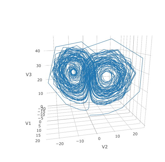
Plotly is much prettier!
Option Handling
If we want to have a more accurate solution, we can send abstol and reltol. Defaults are 1e-6 and 1e-3 respectively.
Generally you can think of the digits of accuracy as related to 1 plus the exponent of the relative tolerance, so the default is
two digits of accuracy. Absolute tolernace is the accuracy near 0.
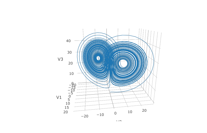
In addition, we may want to choose to save at more time points. We do this by giving an array of values to save at as saveat.
Together, this looks like:
abstol <- 1e-8
reltol <- 1e-8
saveat <- 0:10000/100
sol <- de$solve(prob,abstol=abstol,reltol=reltol,saveat=saveat)
udf <- as.data.frame(t(sapply(sol$u,identity)))
plotly::plot_ly(udf, x = ~V1, y = ~V2, z = ~V3, type = 'scatter3d', mode = 'lines')
We can also choose to use a different algorithm. The choice is done using a string that matches the Julia syntax. See
the ODE tutorial for details.
The list of choices for ODEs can be found at the ODE Solvers page.
For example, let's use a 9th order method due to Verner:
sol <- de$solve(prob,de$Vern9(),abstol=abstol,reltol=reltol,saveat=saveat)
Note that each algorithm choice will cause a JIT compilation
Performance Enhancements
One way to enhance the performance of your code is to define the function in Julia
so that way it is JIT compiled. diffeqr is built using
the JuliaCall package, and so
you can utilize the Julia JIT compiler. We expose this automatically over ODE
functions via jitoptimize_ode, like in the following example:
f <- function(u,p,t) {
  du1 = p[1]*(u[2]-u[1])
  du2 = u[1]*(p[2]-u[3]) - u[2]
  du3 = u[1]*u[2] - p[3]*u[3]
  return(c(du1,du2,du3))
}
u0 <- c(1.0,0.0,0.0)
tspan <- c(0.0,100.0)
p <- c(10.0,28.0,8/3)
prob <- de$ODEProblem(f, u0, tspan, p)
fastprob <- diffeqr::jitoptimize_ode(de,prob)
sol <- de$solve(fastprob,de$Tsit5())
Note that the first evaluation of the function will have an ~2 second lag since
the compiler will run, and all subsequent runs will be orders of magnitude faster
than the pure R function. This means it's great for expensive functions (ex. large
PDEs) or functions called repeatedly, like during optimization of parameters.
We can also use the JuliaCall functions to directly define the function in Julia
to eliminate the R interpreter overhead and get full JIT compilation:
julf <- JuliaCall::julia_eval("
function julf(du,u,p,t)
  du[1] = 10.0*(u[2]-u[1])
  du[2] = u[1]*(28.0-u[3]) - u[2]
  du[3] = u[1]*u[2] - (8/3)*u[3]
end")
JuliaCall::julia_assign("u0", u0)
JuliaCall::julia_assign("p", p)
JuliaCall::julia_assign("tspan", tspan)
prob3 = JuliaCall::julia_eval("ODEProblem(julf, u0, tspan, p)")
sol = de$solve(prob3,de$Tsit5())
To demonstrate the performance advantage, let's time them all:
> system.time({ for (i in 1:100){ de$solve(prob    ,de$Tsit5()) }})
   user  system elapsed
   6.69    0.06    6.78
> system.time({ for (i in 1:100){ de$solve(fastprob,de$Tsit5()) }})
   user  system elapsed
   0.11    0.03    0.14
> system.time({ for (i in 1:100){ de$solve(prob3   ,de$Tsit5()) }})
   user  system elapsed
   0.14    0.02    0.15
This is about a 50x improvement!
JuliaDiffEq/diffeqr documentation built on March 19, 2024, 8:41 p.m.
R Package Documentation
Browse R Packages
We want your feedback!
Note that we can't provide technical support on individual packages. You should contact the package authors for that.
knitr::opts_chunk$set( collapse = TRUE, comment = "#>" )
1D Linear ODEs
Let's solve the linear ODE u'=1.01u. First setup the package:
de <- diffeqr::diffeq_setup()
Define the derivative function f(u,p,t).
f <- function(u,p,t) { return(1.01*u) }
Then we give it an initial condition and a time span to solve over:
u0 <- 1/2 tspan <- c(0., 1.)
With those pieces we define the ODEProblem and solve the ODE:
prob = de$ODEProblem(f, u0, tspan) sol = de$solve(prob)
This gives back a solution object for which sol$t are the time points
and sol$u are the values. We can treat the solution as a continuous object
in time via
and a high order interpolation will compute the value at t=0.2. We can check
the solution by plotting it:
plot(sol$t,sol$u,"l")
Systems of ODEs
Now let's solve the Lorenz equations. In this case, our initial condition is a vector and our derivative functions takes in the vector to return a vector (note: arbitrary dimensional arrays are allowed). We would define this as:
f <- function(u,p,t) { du1 = p[1]*(u[2]-u[1]) du2 = u[1]*(p[2]-u[3]) - u[2] du3 = u[1]*u[2] - p[3]*u[3] return(c(du1,du2,du3)) }
Here we utilized the parameter array p. Thus we use diffeqr::ode.solve like before, but also pass in parameters this time:
u0 <- c(1.0,0.0,0.0) tspan <- list(0.0,100.0) p <- c(10.0,28.0,8/3) prob <- de$ODEProblem(f, u0, tspan, p) sol <- de$solve(prob)
The returned solution is like before except now sol$u is an array of arrays,
where sol$u[i] is the full system at time sol$t[i]. It can be convenient to
turn this into an R matrix through sapply:
mat <- sapply(sol$u,identity)
This has each row as a time series. t(mat) makes each column a time series.
It is sometimes convenient to turn the output into a data.frame which is done
via:
udf <- as.data.frame(t(mat))
Now we can use matplot to plot the timeseries together:
matplot(sol$t,udf,"l",col=1:3)
Now we can use the Plotly package to draw a phase plot:
plotly::plot_ly(udf, x = ~V1, y = ~V2, z = ~V3, type = 'scatter3d', mode = 'lines')
Plotly is much prettier!
Option Handling
If we want to have a more accurate solution, we can send abstol and reltol. Defaults are 1e-6 and 1e-3 respectively.
Generally you can think of the digits of accuracy as related to 1 plus the exponent of the relative tolerance, so the default is
two digits of accuracy. Absolute tolernace is the accuracy near 0.
In addition, we may want to choose to save at more time points. We do this by giving an array of values to save at as saveat.
Together, this looks like:
abstol <- 1e-8 reltol <- 1e-8 saveat <- 0:10000/100 sol <- de$solve(prob,abstol=abstol,reltol=reltol,saveat=saveat) udf <- as.data.frame(t(sapply(sol$u,identity))) plotly::plot_ly(udf, x = ~V1, y = ~V2, z = ~V3, type = 'scatter3d', mode = 'lines')
We can also choose to use a different algorithm. The choice is done using a string that matches the Julia syntax. See the ODE tutorial for details. The list of choices for ODEs can be found at the ODE Solvers page. For example, let's use a 9th order method due to Verner:
sol <- de$solve(prob,de$Vern9(),abstol=abstol,reltol=reltol,saveat=saveat)
Note that each algorithm choice will cause a JIT compilation
Performance Enhancements
One way to enhance the performance of your code is to define the function in Julia
so that way it is JIT compiled. diffeqr is built using
the JuliaCall package, and so
you can utilize the Julia JIT compiler. We expose this automatically over ODE
functions via jitoptimize_ode, like in the following example:
f <- function(u,p,t) { du1 = p[1]*(u[2]-u[1]) du2 = u[1]*(p[2]-u[3]) - u[2] du3 = u[1]*u[2] - p[3]*u[3] return(c(du1,du2,du3)) } u0 <- c(1.0,0.0,0.0) tspan <- c(0.0,100.0) p <- c(10.0,28.0,8/3) prob <- de$ODEProblem(f, u0, tspan, p) fastprob <- diffeqr::jitoptimize_ode(de,prob) sol <- de$solve(fastprob,de$Tsit5())
Note that the first evaluation of the function will have an ~2 second lag since the compiler will run, and all subsequent runs will be orders of magnitude faster than the pure R function. This means it's great for expensive functions (ex. large PDEs) or functions called repeatedly, like during optimization of parameters.
We can also use the JuliaCall functions to directly define the function in Julia to eliminate the R interpreter overhead and get full JIT compilation:
julf <- JuliaCall::julia_eval(" function julf(du,u,p,t) du[1] = 10.0*(u[2]-u[1]) du[2] = u[1]*(28.0-u[3]) - u[2] du[3] = u[1]*u[2] - (8/3)*u[3] end") JuliaCall::julia_assign("u0", u0) JuliaCall::julia_assign("p", p) JuliaCall::julia_assign("tspan", tspan) prob3 = JuliaCall::julia_eval("ODEProblem(julf, u0, tspan, p)") sol = de$solve(prob3,de$Tsit5())
To demonstrate the performance advantage, let's time them all:
> system.time({ for (i in 1:100){ de$solve(prob ,de$Tsit5()) }}) user system elapsed 6.69 0.06 6.78 > system.time({ for (i in 1:100){ de$solve(fastprob,de$Tsit5()) }}) user system elapsed 0.11 0.03 0.14 > system.time({ for (i in 1:100){ de$solve(prob3 ,de$Tsit5()) }}) user system elapsed 0.14 0.02 0.15
This is about a 50x improvement!
R Package Documentation
Browse R Packages
We want your feedback!
Note that we can't provide technical support on individual packages. You should contact the package authors for that.
Embedding an R snippet on your website
Add the following code to your website.
For more information on customizing the embed code, read Embedding Snippets.