README.md

In KeesVanImmerzeel/mipwelcona: Calculate The Development Of Concentrations Of Solvents In Pumped Groundwater

Package mipwelcona

The package mipwelcona can be used to calculate the development of the concentrations of solvents in pumped groundwater. The package is based on the results of:

• streamline calculations (backwards from well screens) in a MIPWA groundwater model;
• Initial concentrations in specified layers;
• Levels of concentration layers;
• Parameters of different processes.

This package is a further development of the program WELCONA.

Installation

You can install the released version of menyanthes from with:

devtools::install_github("KeesVanImmerzeel/mipwelcona")

Then load the package with:

library("mipwelcona")

Functions in this package

• mw_read_streamlines(): Read streamlines from *.iff file;
• mw_read_well_filters(): Read wells from *.ipf file;
• mw_conc_init(): Initialize base streamline concentration table;
• mw_conc_streamlines(): Calculate concentrations on streamlines at specified times.
• mw_create_sl_fltr_table(): Create table with indices linking the streamlines to well filters.
• mw_conc_filters(): Calculate concentrations (mixed) of selected filters at times as specified in table created with mw_conc_streamlines()
• mw_conc_wells(): Calculate concentrations (mixed) of selected wells at times as specified in table created with mw_conc_streamlines().

Functions to create example data:

• mw_example_conc_layer_levels(): Initialise example concentration layer levels;
• mw_example_concentrations(): Initialise example concentrations in the subsoil;
• mw_example_base_streamline_conc_table(): Initialise example base streamline concentration table as created with the function mw_conc_init();
• mw_example_conc_streamlines(): Initialise example concentrations on streamlines at specified times as created with function mw_conc_streamlines().
• mw_example_sl_fltr_table(): Initiate example table with indices linking the streamlines to well filters as created with function mw_create_sl_fltr_table().

Get help

To get help on the functions in this package type a question mark before the function name, like ?mw_read_streamlines()

Files needed

Prepare the following files in order to be able to perform an analysis with mipwelcona:

• iff streamline file;
• ipf well filter file;
• For every concentration layer: a map with initial concentrations;
• The levels (relative to a reference level) between these concentration layers.

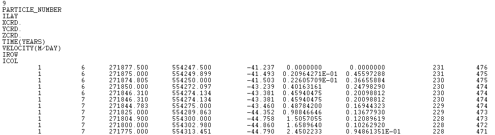
By streamline calculation in MIPWA (backwards from well screens), an iff file is created. Here is a screenshot of the top lines in an iff file containing the calculated streamlines.

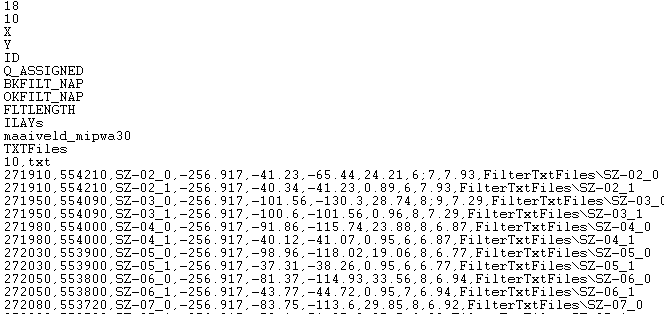
In MIPWA the ipf file specifies the well characteristics (location, discharge etc.). Here is a screenshot of the top lines in an ipf file.

The initial concentrations in the subsoil must be specified for every concentration layer. These initial concentrations (maps) have the format of a RasterLayer. In mipwelcona these raster layers are specified in a single object: a RasterBrick. The first RasterLayer in the RasterBrick represents the concentrations in the top concentration layer, the second RasterLayer represents the concentrations in the concentration layer below the first concentration layer etc. An example of a RasterBrick with concentrations is supplied using the function mw_example_concentrations().

The concentration layers are separated at levels that are also with a RasterBrick object. The first RasterLayer in this RasterBrick represents the levels between the top concentration layer and the concentration layer below the top concentration layer etc. So, if (n) concentration layers are specified, the number of level RasterLayers to specify is equal to (n-1). An example of a RasterBrick with levels of concentration layers is supplied using the function mw_example_conc_layer_levels().

Example work flow

Step 1: read streamlines.

fname <- system.file("extdata","streamlines.iff",package="mipwelcona")

strm_lns <- mw_read_streamlines(fname)

Step 2: Read well filters.

fname <- system.file("extdata","well_filters.ipf",package="mipwelcona")

well_fltrs <- mw_read_well_filters(fname)

Step 3: Create concentration layer levels

(8 example rasters layers in this case).

conc_l_lev <- mw_example_conc_layer_levels()

Step 4: Create Initial concentrations of different layers in the subsoil

(9 example rasters layers in this case).

conc_l <- mw_example_concentrations()

Step 5: Initialize base streamline concentration table.

conc_strm_lns <- mw_conc_init(strm_lns, conc_l_lev, conc_l)

Step 6: Calculate concentrations on streamlines at specified times.

conc_streamlines <- mw_conc_streamlines(conc_strm_lns, times=c(1*365,5*365,10*365,25*365), processes=c("dispersion","decay", "retardation"), alpha=0.3, rho=3, labda=0.0001, retard=1)

Step 7: Create table with indices linking the streamlines to well filters.

# sl_fltr_table <- mw_create_sl_fltr_table(strm_lns, well_fltrs, maxdist=100)

Step 8: Calculate concentrations (mixed) of selected filters or selected wells.

Overrule previously created table first for this example. Normally, you wouln't do this!

sl_fltr_table <- mw_example_sl_fltr_table()

conc <- mw_conc_filters( fltr_nrs=c(1,2), well_fltrs, sl_fltr_table, conc_streamlines )

conc <- mw_conc_wells( well_nrs=c(1,9), well_fltrs, sl_fltr_table, conc_streamlines )

References

The theory behind the concentration calculations is published in Stromingen 1996, Stromingen 1996 (2).

KeesVanImmerzeel/mipwelcona documentation built on Nov. 11, 2020, 10:35 p.m.