In LudvigOlsen/rearrr: Rearranging Data
if (requireNamespace("knitr", quietly = TRUE)){
  knitr::opts_chunk$set(
    collapse = TRUE,
    comment = "#>",
    fig.path = "man/figures/README-",
    dpi = 92,
    fig.retina = 2
  )
}

# Get minimum R requirement
dep <- as.vector(read.dcf('DESCRIPTION')[, 'Depends'])
rvers <- substring(dep, 7, nchar(dep)-1)
# m <- regexpr('R *\\\\(>= \\\\d+.\\\\d+.\\\\d+\\\\)', dep)
# rm <- regmatches(dep, m)
# rvers <- gsub('.*(\\\\d+.\\\\d+.\\\\d+).*', '\\\\1', dep)

# Function for TOC
# https://gist.github.com/gadenbuie/c83e078bf8c81b035e32c3fc0cf04ee8
rearrr
Rearrrange Data
Authors: Ludvig R. Olsen ( r-pkgs@ludvigolsen.dk )

License: MIT
Started: April 2020


Overview
R package for rearranging data by a set of methods.
We distinguish between rearrangers and mutators, where the first reorders the data points and the second changes the values of the data points.
When performing an operation relative to a point in an n-dimensional vector space, we refer to the point as the origin. If we, for instance, wish to rotate our data points around the point at x = 3 and y = 7, those are the coordinates of our origin.
Install
CRAN (when available):
install.packages("rearrr")
Development version:
install.packages("devtools")
devtools::install_github("LudvigOlsen/rearrr")
Rearrangers
| Function | Description |
|:----------------------|:----------------------------------------------------------------------|
|center_max() |Center the highest value with values decreasing around it. |
|center_min() |Center the lowest value with values increasing around it. |
|position_max() |Position the highest value with values decreasing around it. |
|position_min() |Position the lowest value with values increasing around it. |
|pair_extremes() |Arrange as lowest, highest, 2nd lowest, 2nd highest, etc. |
|triplet_extremes() |Arrange as lowest, most middle, highest, 2nd lowest, 2nd most middle, 2nd highest, etc. |
|closest_to() |Order values by shortest distance to an origin. |
|furthest_from() |Order values by longest distance to an origin. |
|rev_windows() |Reverse order window-wise. |
|roll_elements() |Rolls/shifts positions of elements. |
|shuffle_hierarchy() |Shuffle multi-column hierarchy of groups. |
Mutators
| Function | Description | Dimensions |
|:----------------------|:----------------------------------------------------------------------|:-----------|
|rotate_2d(), rotate_3d() |Rotate values around an origin in 2 or 3 dimensions. |2 or 3 |
|swirl_2d(), swirl_3d() |Swirl values around an origin in 2 or 3 dimensions. |2 or 3 |
|shear_2d(), shear_3d() |Shear values around an origin in 2 or 3 dimensions. |2 or 3 |
|expand_distances() |Expand distances to an origin. |n |
|expand_distances_each()|Expand distances to an origin separately for each dimension. |n |
|cluster_groups() |Move data points into clusters around group centroids. |n |
|dim_values() |Dim values of a dimension by the distance to an n-dimensional origin. |n (alters 1)|
|flip_values() |Flip the values around an origin. |n |
|roll_values() |Shifts values and wraps to a range. |n |
|wrap_to_range() |Wraps values to a range. |n |
|transfer_centroids() |Transfer centroids from one data.frame to another. |n |
|apply_transformation_matrix() |Apply transformation matrix to data.frame columns. |n |
Formers
| Function | Description |
|:------------------|:----------------------------------------------------------------------|
|circularize() |Create x-coordinates for y-coordinates so they form a circle. |
|hexagonalize() |Create x-coordinates for y-coordinates so they form a hexagon. |
|square() |Create x-coordinates for y-coordinates so they form a square. |
|triangularize() |Create x-coordinates for y-coordinates so they form a triangle. |
Pipelines
| Class | Description |
|:---------------------|:------------------------------------------------------------------------|
|Pipeline |Chain multiple transformations. |
|GeneratedPipeline |Chain multiple transformations and generate argument values per group. |
|FixedGroupsPipeline |Chain multiple transformations with different argument values per group. |
Generators
| Function | Description |
|:----------------------|:----------------------------------------------------------------------|
|generate_clusters() |Generate n-dimensional clusters. |
Additionally, some functions have *_vec() versions, that take and return a vector.
Note: The available utility functions (like scalers, converters and measuring functions) are
listed at the bottom of the readme.
Table of Contents
rearrr:::render_toc("README.Rmd", toc_depth = 4)
Attach packages
Let's see some examples. We start by attaching the necessary packages:
library(rearrr)
library(dplyr)

xpectr::set_test_seed(1)
library(knitr)        # kable()
has_tidyr <- require(tidyr)        # gather()
has_ggplot <- require(ggplot2)  # Attach if installed

vec <- 1:10
random_sample <- runif(10)
orderings <- data.frame(
  "Position" = as.integer(vec),
  "center_max" = center_max(vec),
  "center_min" = center_min(vec),
  "position_max" = position_max(vec, position = 3),
  "position_min" = position_min(vec, position = 3),
  "pair_extremes" = pair_extremes_vec(vec),
  "rev_windows" = rev_windows_vec(vec, window_size = 3),
  "closest_to" = closest_to_vec(vec, origin_fn = create_origin_fn(median)),
  "furthest_from" = furthest_from_vec(vec, origin = 5),
  "random_sample" = random_sample,
  "flipped_median" = flip_values_vec(random_sample, origin_fn=create_origin_fn(median)),
  stringsAsFactors = FALSE
)

# Convert to long format for plotting
if (has_tidyr){
  orderings <- orderings %>%
    tidyr::gather(key = "Method", value = "Value", 2:(ncol(orderings)))
}

gg_line_alpha <- .4
gg_base_line_size <- .3
While we can use the functions with data.frames, we showcase many of them with a vector for simplicity.
At times, we use the *_vec() version of a function in order to get the output as a vector instead of a data.frame.
The functions work with grouped data.frames and in magrittr pipelines (%>%).
Rearranger examples
Rearrangers change the order of the data points.
Center min/max
center_max(data = 1:10)
center_min(data = 1:10)
if (has_ggplot && has_tidyr){

  # Plot centering methods
  orderings %>%
    dplyr::filter(Method %in% c("center_min", "center_max")) %>%
    ggplot(aes(x = Position, y = Value, color = Method)) +
    geom_line(alpha = gg_line_alpha) +
    geom_point() +
    theme_minimal(base_line_size = gg_base_line_size) +
    scale_x_continuous(breaks = c(2, 4, 6, 8, 10)) +
    scale_y_continuous(breaks = c(2, 4, 6, 8, 10)) +
    scale_colour_brewer(palette = "Dark2")

}
Position min/max
position_max(data = 1:10, position = 3)
position_min(data = 1:10, position = 3)
if (has_ggplot && has_tidyr){

  # Plot positioning methods
  orderings %>%
    dplyr::filter(Method %in% c("position_min", "position_max")) %>%
    ggplot(aes(x = Position, y = Value, color = Method)) +
    geom_line(alpha = gg_line_alpha) +
    geom_point() +
    theme_minimal(base_line_size = gg_base_line_size) +
    scale_x_continuous(breaks = c(2, 4, 6, 8, 10)) +
    scale_y_continuous(breaks = c(2, 4, 6, 8, 10)) +
    scale_colour_brewer(palette = "Dark2")

}
Pair extremes
pair_extremes(data = 1:10)
if (has_ggplot && has_tidyr){

  # Plot extreme pairing
  orderings %>%
    dplyr::filter(Method == "pair_extremes") %>%
    ggplot(aes(x = Position, y = Value, color = Method)) +
    geom_line(alpha = gg_line_alpha) +
    geom_point() +
    theme_minimal(base_line_size = gg_base_line_size) +
    scale_x_continuous(breaks = c(2, 4, 6, 8, 10)) +
    scale_y_continuous(breaks = c(2, 4, 6, 8, 10)) +
    scale_colour_brewer(palette = "Dark2")

}
Closest to / furthest from
We use the _vec() versions to get the reordered vectors. For data.frames, use closest_to()/furthest_from() instead.
The origin can be passed as either a specific coordinate (here, a value in data) or a function.
closest_to_vec(data = 1:10, origin_fn = create_origin_fn(median))
furthest_from_vec(data = 1:10, origin = 5)
if (has_ggplot && has_tidyr){

  # Plot distanced order
  orderings %>%
    dplyr::filter(Method %in% c("closest_to", "furthest_from")) %>%
    ggplot(aes(x = Position, y = Value, color = Method)) +
    geom_line(alpha = gg_line_alpha) +
    geom_point() +
    theme_minimal(base_line_size = gg_base_line_size) +
    scale_x_continuous(breaks = c(2, 4, 6, 8, 10)) +
    scale_y_continuous(breaks = c(2, 4, 6, 8, 10)) +
    scale_colour_brewer(palette = "Dark2")

}
Reverse windows
We use the _vec() version to get the reordered vector. For data.frames, use rev_windows() instead.
rev_windows_vec(data = 1:10, window_size = 3)
if (has_ggplot && has_tidyr){

  # Plot windowed reversing
  orderings %>%
    dplyr::filter(Method == "rev_windows") %>%
    ggplot(aes(x = Position, y = Value, color = Method)) +
    geom_line(alpha = gg_line_alpha) +
    geom_point() +
    theme_minimal(base_line_size = gg_base_line_size) +
    scale_x_continuous(breaks = c(2, 4, 6, 8, 10)) +
    scale_y_continuous(breaks = c(2, 4, 6, 8, 10)) +
    scale_colour_brewer(palette = "Dark2")

}
Shuffle Hierarchy
When having a data.frame with multiple grouping columns, we can shuffle them one column (hierarchical level) at a time:
# Shuffle a given data frame 'df'
shuffle_hierarchy(df, group_cols = c("a", "b", "c"))
The columns are shuffled one at a time, as so:
Mutator examples
Mutators change the values of the data points.
Rotate values
2-dimensional rotation:
# Set seed for reproducibility
xpectr::set_test_seed(1)

# Draw random numbers
random_sample <- round(runif(10), digits = 4)
random_sample

rotate_2d(
  data = random_sample,
  degrees = 60,
  origin_fn = centroid
)
rotate_df <- rotate_2d(random_sample, degrees = c(0, 72, 144, 216, 288), origin_fn = centroid)

if (has_ggplot){

  # Plot rotated values
  rotate_df %>%
    ggplot(aes(x = Index_rotated, y = Value_rotated, color = factor(.degrees))) +
    geom_hline(yintercept = mean(random_sample), size = 0.2, alpha = gg_line_alpha, linetype="dashed") +
    geom_vline(xintercept = mean(seq_len(length(random_sample))), size = 0.2, alpha = gg_line_alpha, linetype="dashed") +
    geom_path(alpha = gg_line_alpha) +
    geom_point() +
    theme_minimal(base_line_size = gg_base_line_size) +
    scale_colour_brewer(palette = "Dark2") +
    labs(x = "Index", y="Value", color="Degrees")

}
3-dimensional rotation:
# Set seed
set.seed(3)

# Create a data frame
df <- data.frame(
  "x" = 1:12,
  "y" = c(1, 2, 3, 4, 9, 10, 11,
          12, 15, 16, 17, 18),
  "z" = runif(12)
)

# Perform rotation
rotate_3d(
  data = df,
  x_col = "x",
  y_col = "y",
  z_col = "z",
  x_deg = 45,
  y_deg = 90,
  z_deg = 135,
  origin_fn = centroid
)
rotate_df <- df %>%
  rotate_3d(x_col = "x",
           y_col = "y",
           z_col = "z",
           x_deg = c(0, 72, 144, 216, 288),
           y_deg = c(0, 72, 144, 216, 288),
           z_deg = c(0, 72, 144, 216, 288),
           origin_fn = centroid)

if (has_ggplot){

  # Plot rotated values
  rotate_df %>%
    ggplot(aes(x = x_rotated, y = y_rotated, color = .degrees_str, alpha = z_rotated)) +
    geom_vline(xintercept = mean(df$x), size = 0.2, alpha = .4, linetype="dashed") +
    geom_hline(yintercept = mean(df$y), size = 0.2, alpha = .4, linetype="dashed") +
    geom_path(alpha = gg_line_alpha) +
    geom_point() +
    theme_minimal(base_line_size = gg_base_line_size) +
    scale_colour_brewer(palette = "Dark2") +
    labs(x = "x", y = "y", color = "degrees", alpha = "z (opacity)")

}
Swirl values
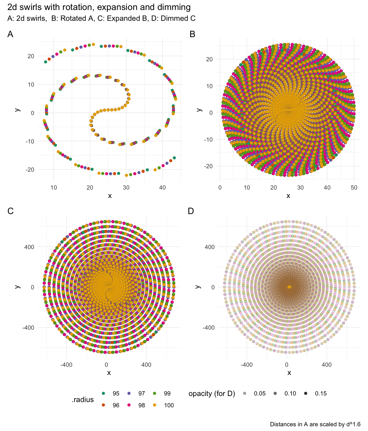
2-dimensional swirling:
# Rotate values
swirl_2d(data = rep(1, 50), radius = 95, origin = c(0, 0))
# Swirl around the centroid
df_swirled <- swirl_2d(
  data = rep(1, 50),
  radius = c(95, 96, 97, 98, 99, 100),
  origin_fn = centroid,
  suffix = "",
  scale_fn = function(x) {
    x ^ 1.6
  }
)

orig <- df_swirled$.origin[[1]]

if (has_ggplot){

  # Plot swirls
  ggswirl1 <- df_swirled %>%
    ggplot(aes(x = Index, y = Value, color = factor(.radius))) +
    geom_point() +
    theme_minimal(base_line_size = gg_base_line_size) +
    scale_colour_brewer(palette = "Dark2") +
    labs(x = "x", y = "y", color = ".radius")

}

df_swirled <- df_swirled %>%
  rotate_2d(degrees = (1:36) * 10,
           x_col = "Index",
           y_col = "Value",
           suffix = "",
           origin = orig)

if (has_ggplot){

  # Plot rotated swirls
  ggswirl2 <- df_swirled %>%
    ggplot(aes(x = Index, y = Value, color = factor(.radius))) +
    geom_point() +
    theme_minimal(base_line_size = gg_base_line_size) +
    scale_colour_brewer(palette = "Dark2") +
    labs(x = "x", y = "y", color = ".radius")

}

# Expand values ^2
df_swirled <- df_swirled %>%
  expand_distances(
    cols = c("Index", "Value"),
    multiplier = 2,
    exponentiate = T,
    origin = orig,
    suffix = "")

if (has_ggplot){

  # Plot expanded swirls
  ggswirl3 <- df_swirled %>%
    ggplot(aes(x = Index, y = Value, color = factor(.radius))) +
    geom_point() +
    theme_minimal(base_line_size = gg_base_line_size) +
    scale_colour_brewer(palette = "Dark2") +
    labs(x = "x", y = "y", color = ".radius")

}

# Dim values
df_swirled <- df_swirled %>%
  mutate(o = 1) %>%
  dim_values(cols = c("Index", "Value", "o"), origin = c(orig, 1), suffix = "")

if (has_ggplot){

  # Plot rotated swirls
  ggswirl4 <- df_swirled %>%
    ggplot(aes(x = Index, y = Value, alpha = o, color = factor(.radius))) +
    geom_point() +
    theme_minimal(base_line_size = gg_base_line_size) +
    scale_colour_brewer(palette = "Dark2") +
    labs(x = "x", y = "y", color = ".radius", alpha = "opacity (for D)")

  combined <- (ggswirl1 + ggswirl2) / (ggswirl3 + ggswirl4) & theme(legend.position = "bottom")
  combined <- combined + plot_layout(guides = "collect")
  combined +
    plot_annotation(title = "2d swirls with rotation, expansion and dimming",
                    subtitle = "A: 2d swirls,  B: Rotated A, C: Expanded B, D: Dimmed C",
                    caption = "Distances in A are scaled by d^1.6",
                    tag_levels = 'A')

}
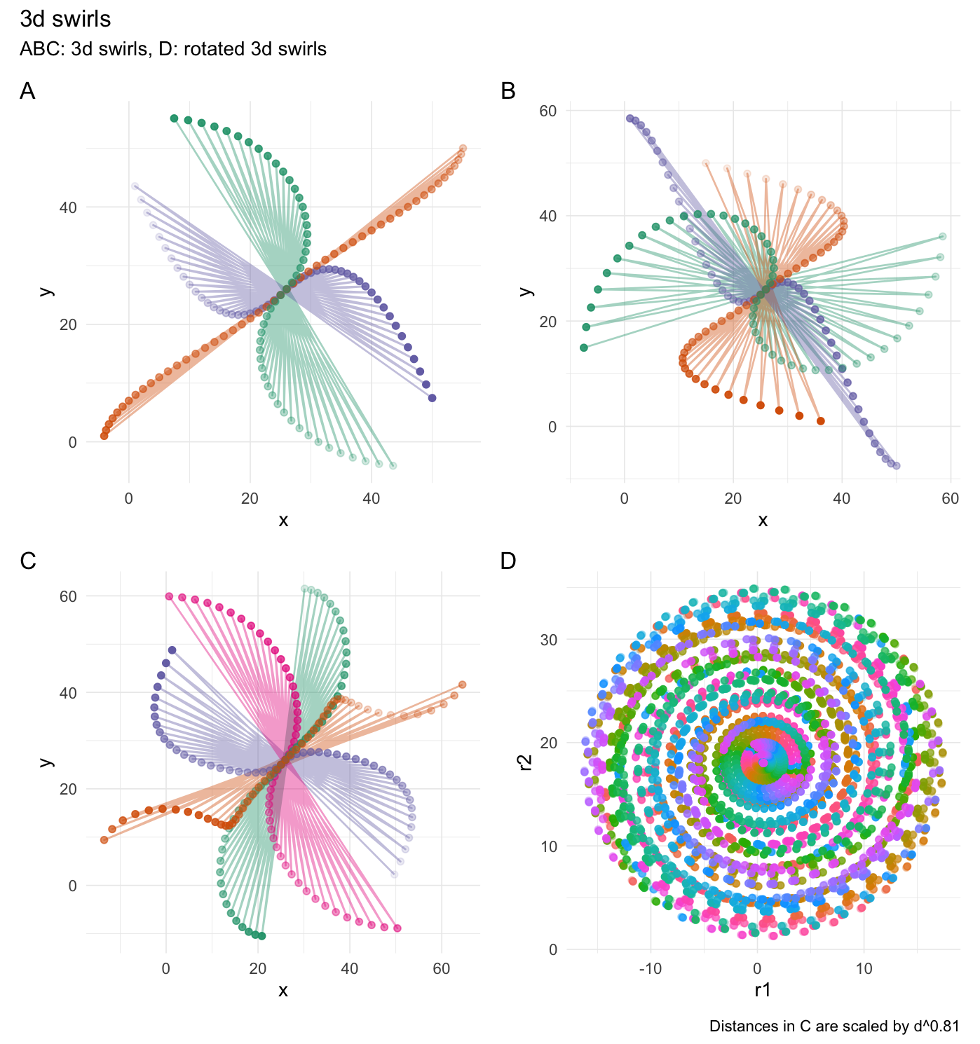
3-dimensional swirling:
# Set seed
set.seed(4)

# Create a data frame
df <- data.frame(
  "x" = 1:50,
  "y" = 1:50,
  "z" = 1:50,
  "r1" = runif(50),
  "r2" = runif(50) * 35,
  "o" = 1,
  "g" = rep(1:5, each = 10)
)

# They see me swiiirling
swirl_3d(
  data = df,
  x_radius = 45,
  x_col = "x",
  y_col = "y",
  z_col = "z",
  origin = c(0, 0, 0),
  keep_original = FALSE
)
# 1st plot

df_swirled <- swirl_3d(
  data = df,
  x_col = "x",
  y_col = "y",
  z_col = "z",
  x_radius = c(100, 0, 0),
  y_radius = c(0, 100, 0),
  z_radius = c(0, 0, 100),
  origin_fn = centroid
)

if (has_ggplot){

  ggswirl_3d_1 <- df_swirled %>%
    ggplot(aes(x = x_swirled, y = y_swirled, color = .radius_str, alpha = z_swirled)) +
    geom_path(alpha = gg_line_alpha) +
    geom_point() +
    theme_minimal(base_line_size = gg_base_line_size) +
    scale_colour_brewer(palette = "Dark2") +
    labs(x = "x", y = "y", color = "radius", alpha = "z (opacity)")

}


# 2nd plot

df_swirled <- swirl_3d(
  data = df,
  x_col = "x",
  y_col = "y",
  z_col = "z",
  x_radius = c(50, 0, 0),
  y_radius = c(0, 50, 0),
  z_radius = c(0, 0, 50),
  origin_fn = centroid
)

if (has_ggplot){

  ggswirl_3d_2 <- df_swirled %>%
    ggplot(aes(x = x_swirled, y = y_swirled, color = .radius_str, alpha = z_swirled)) +
    geom_path(alpha = gg_line_alpha) +
    geom_point() +
    theme_minimal(base_line_size = gg_base_line_size) +
    scale_colour_brewer(palette = "Dark2") +
    labs(x = "x", y = "y", color = "radius", alpha = "z (opacity)")

}

# 3rd plot

df_swirled <- swirl_3d(
  data = df,
  x_col = "x",
  y_col = "y",
  z_col = "z",
  x_radius = c(25, 50, 25, 25),
  y_radius = c(50, 75, 100, 25),
  z_radius = c(75, 25, 25, 25),
  origin_fn = centroid,
  scale_fn = function(x) {
    x^0.81
  }
)

if (has_ggplot){

  ggswirl_3d_3 <- df_swirled %>%
    ggplot(aes(x = x_swirled, y = y_swirled, color = .radius_str, alpha = z_swirled)) +
    geom_path(alpha = gg_line_alpha) +
    geom_point() +
    theme_minimal(base_line_size = gg_base_line_size) +
    scale_colour_brewer(palette = "Dark2") +
    labs(x = "x", y = "y", color = "radius", alpha = "z (opacity)")

}

# 4th plot

df_swirled <- swirl_3d(
  data = df,
  x_col = "r1",
  y_col = "r2",
  z_col = "o",
  x_radius = c(0, 0, 0, 0),
  y_radius = c(0, 30, 60, 90),
  z_radius = c(10, 10, 10, 10),
  origin_fn = centroid
)

# Not let's rotate it every 10 degrees
df_rotated <- df_swirled %>%
  rotate_3d(
    x_col = "r1_swirled",
    y_col = "r2_swirled",
    z_col = "o_swirled",
    x_deg = rep(0, 36),
    y_deg = rep(0, 36),
    z_deg = (1:36) * 10,
    suffix = "",
    origin = df_swirled$.origin[[1]])

if (has_ggplot){

  ggswirl_3d_4 <- df_rotated %>%
    ggplot(aes(x = r1_swirled, y = r2_swirled, color = .degrees_str,  alpha = o_swirled)) +
    geom_point(show.legend = FALSE) +
    theme_minimal(base_line_size = gg_base_line_size) +
    # scale_colour_brewer(palette = "Dark2") +
    labs(x = "r1", y = "r2", color = "radius", alpha = "o (opacity)")

  combined <- (ggswirl_3d_1 + ggswirl_3d_2) / (ggswirl_3d_3 + ggswirl_3d_4) & theme(legend.position = "none")
  # combined <- combined + plot_layout(guides = "collect")
  combined +
    plot_annotation(title = "3d swirls",
                    subtitle = "ABC: 3d swirls, D: rotated 3d swirls",
                    caption = "Distances in C are scaled by d^0.81",
                    tag_levels = 'A')

}
Expand distances
# 1d expansion
expand_distances(
  data = random_sample,
  multiplier = 3,
  origin_fn = centroid,
  exponentiate = TRUE
)
2d expansion:
xpectr::set_test_seed(36)
random_x <- runif(10)
random_y <- runif(10)
expand_df <- purrr::map_dfr(
  .x = c(1, 2, 3, 4, 5),
  .f = function(exponent) {
    expand_distances(
      data.frame("x" = random_x,
                 "y" = random_y),
      cols = c("x", "y"),
      multiplier = exponent,
      origin_fn = centroid,
      exponentiate = TRUE
    )
  }
)

if (has_ggplot){

  # Plot rotated values
  expand_df %>%
    ggplot(aes(x = x_expanded, y = y_expanded, color = factor(.exponent))) +
    geom_hline(yintercept = mean(random_y), size = 0.2, alpha = gg_line_alpha, linetype="dashed") +
    geom_vline(xintercept = mean(random_x), size = 0.2, alpha = gg_line_alpha, linetype="dashed") +
    geom_path(alpha = gg_line_alpha) +
    geom_point() +
    theme_minimal(base_line_size = gg_base_line_size) +
    scale_colour_brewer(palette = "Dark2") +
    labs(x = "x", y="y", color="Exponent")

}

xpectr::set_test_seed(36) # for next section
Expand differently in each axis:
# Expand x-axis and contract y-axis
expand_distances_each(
  data.frame("x" = runif(10),
             "y" = runif(10)),
  cols = c("x", "y"),
  multipliers = c(7, 0.5),
  origin_fn = centroid
)
rand_df <- data.frame("x" = random_x,
                      "y" = random_y)
expand_df <- purrr::map2_dfr(
  .x = c(7, 1),
  .y = c(0.5, 1),
  .f = function(m1, m2) {
    expand_distances_each(
      rand_df,
      cols = c("x", "y"),
      multipliers = c(m1, m2),
      origin_fn = centroid
    )
  }
)

if (has_ggplot){

  # Plot rotated values
  expand_df %>%
    ggplot(aes(x = x_expanded, y = y_expanded, color = factor(.multipliers_str))) +
    geom_hline(yintercept = mean(random_y), size = 0.2, alpha = gg_line_alpha, linetype = "dashed") +
    geom_vline(xintercept = mean(random_x), size = 0.2, alpha = gg_line_alpha, linetype = "dashed") +
    geom_path(alpha = gg_line_alpha) +
    geom_point() +
    theme_minimal(base_line_size = gg_base_line_size) +
    scale_colour_brewer(palette = "Dark2") +
    labs(x = "x", y = "y", color = "Multiplier")

}
Cluster groups
# Set seed for reproducibility
xpectr::set_test_seed(3)

# Create data frame with random data and a grouping variable
df <- data.frame(
  "x" = runif(50),
  "y" = runif(50),
  "g" = rep(c(1, 2, 3, 4, 5), each = 10)
)

cluster_groups(
  data = df,
  cols = c("x", "y"),
  group_col = "g"
)
df_clustered <- cluster_groups(df, cols = c("x", "y"), group_col = "g")

if (has_ggplot){

  ggplot(df_clustered, aes(x = x_clustered, y = y_clustered, color = factor(g))) +
    # Original data
    geom_point(aes(x = x, y = y), alpha = 0.3, size = 0.8) +
    # Clustered data
    geom_point() +
    theme_minimal(base_line_size = gg_base_line_size) +
    scale_colour_brewer(palette = "Dark2") +
    labs(x = "x", y = "y", color = "g", caption = "Semi-transparent points are the original data points.")

}

df_clustered <- df_clustered %>%
  dplyr::select(x_clustered, y_clustered, g)
Dim values
# Add a column with 1s
df_clustered$o <- 1

# Dim the "o" column based on the data point's distance
# to the most central point in the cluster
df_clustered %>%
  dplyr::group_by(g) %>%
  dim_values(
    cols = c("x_clustered", "y_clustered"),
    dim_col = "o",
    origin_fn = most_centered
  )
df_dimmed <- df_clustered %>%
  dplyr::group_by(g) %>%
  dim_values(cols = c("x_clustered", "y_clustered", "o"), origin_fn = most_centered)

if (has_ggplot){

  ggplot(df_dimmed, aes(x = x_clustered, y = y_clustered, alpha = o_dimmed, color = factor(g))) +
    geom_point() +
    theme_minimal(base_line_size = gg_base_line_size) +
    scale_colour_brewer(palette = "Dark2") +
    labs(x = "x", y = "y", color = "g", alpha = "o_dimmed")

}
Flip values
# The median value to flip around
median(random_sample)

# Flip the random numbers around the median
flip_values(
  data = random_sample,
  origin_fn = create_origin_fn(median)
)
if (has_ggplot && has_tidyr){

  # Plot flipped values
  orderings %>%
    dplyr::filter(Method %in% c("random_sample", "flipped_median")) %>%
    ggplot(aes(x = Position, y = Value, color = Method)) +
    geom_line(alpha = gg_line_alpha) +
    geom_point() +
    theme_minimal(base_line_size = gg_base_line_size) +
    scale_x_continuous(breaks = c(2, 4, 6, 8, 10)) +
    scale_colour_brewer(palette = "Dark2")

}
Forming examples
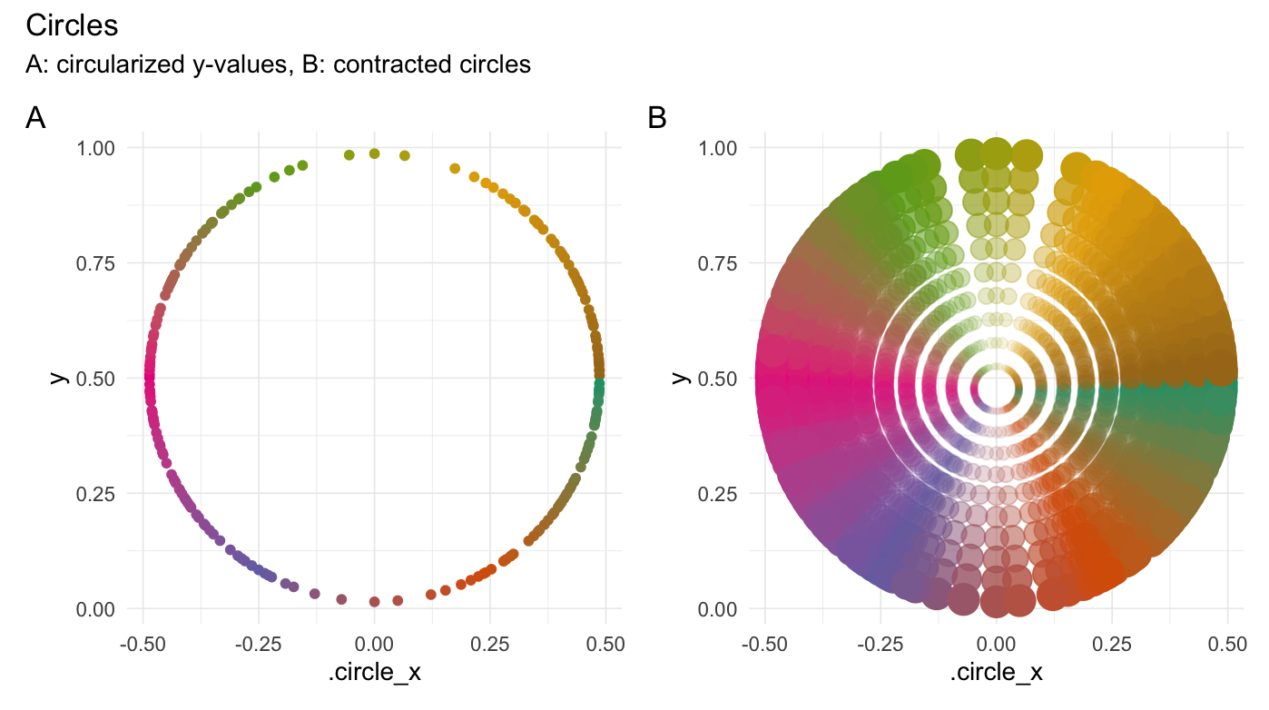
Circularize points
circularize(runif(200))
xpectr::set_test_seed(10)

# Create a data frame
df <- data.frame(
  "y" = runif(200)
)

df_circ <- circularize(df, y_col = "y")

if (has_ggplot){

  ggcirc_1 <- df_circ %>%
    ggplot(aes(x = .circle_x, y = y, color = .degrees)) +
    geom_point() +
    theme_minimal(base_line_size = gg_base_line_size) +
    scale_colour_distiller(palette = "Dark2") +
    labs(x = ".circle_x", y = "y")

}

df_circ_expanded <- purrr::map_dfr(
  .x = 1:10/10,
  .f = function(mult){
    expand_distances(
      data = df_circ,
      cols = c(".circle_x", "y"),
      multiplier = mult,
      origin_fn = centroid)
  })

if (has_ggplot){

  ggcirc_2 <- df_circ_expanded %>%
    ggplot(aes(x = .circle_x_expanded, y = y_expanded,
               color = .degrees, alpha = 0.8*.multiplier^2)) +
    geom_point(aes(size = 0.8*.multiplier^2)) +
    theme_minimal(base_line_size = gg_base_line_size) +
    scale_colour_distiller(palette = "Dark2") +
    labs(x = ".circle_x", y = "y")

  combined <- (ggcirc_1 + ggcirc_2) & theme(legend.position = "none")
  combined +
    plot_annotation(title = "Circles",
                    subtitle = "A: circularized y-values, B: contracted circles",
                    tag_levels = 'A')

}
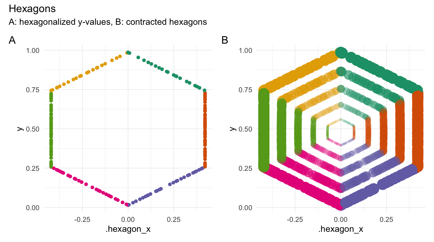
Hexagonalize points
hexagonalize(runif(200))
xpectr::set_test_seed(10)

# Create a data frame
df <- data.frame(
  "y" = runif(200)
)

df_hex <- hexagonalize(df, y_col = "y")

if (has_ggplot){

  gghex_1 <- df_hex %>%
    ggplot(aes(x = .hexagon_x, y = y, color = .edge)) +
    geom_point() +
    theme_minimal(base_line_size = gg_base_line_size) +
    scale_colour_brewer(palette = "Dark2") +
    labs(x = ".hexagon_x", y = "y")

}

df_hex_expanded <- purrr::map_dfr(
  .x = 1:5/10*2,
  .f = function(mult){
    expand_distances(
      data = df_hex,
      cols = c(".hexagon_x", "y"),
      multiplier = mult,
      exponentiate = TRUE,
      origin_fn = centroid)
  })

if (has_ggplot){

  gghex_2 <- df_hex_expanded %>%
    ggplot(aes(x = .hexagon_x_expanded, y = y_expanded,
               color = .edge, alpha = 0.8*.exponent^2)) +
    geom_point(aes(size = 0.8*.exponent^2)) +
    theme_minimal(base_line_size = gg_base_line_size) +
    scale_colour_brewer(palette = "Dark2") +
    labs(x = ".hexagon_x", y = "y")

  combined <- (gghex_1 + gghex_2) & theme(legend.position = "none")
  combined +
    plot_annotation(title = "Hexagons",
                    subtitle = "A: hexagonalized y-values, B: contracted hexagons",
                    tag_levels = 'A')

}
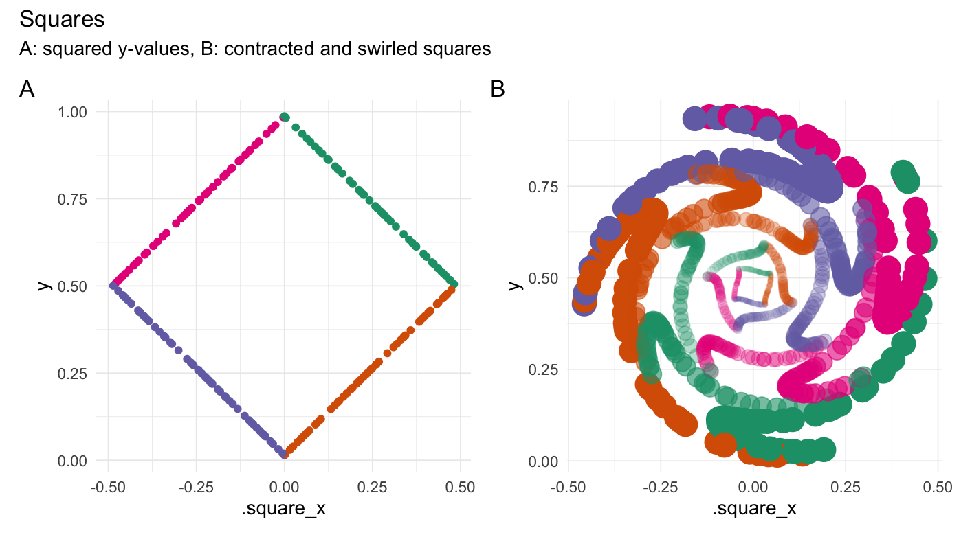
Square points
square(runif(200))
df_sq <- square(df, y_col = "y")

if (has_ggplot){

  ggsq_1 <- df_sq %>%
    ggplot(aes(x = .square_x, y = y, color = .edge)) +
    geom_point() +
    theme_minimal(base_line_size = gg_base_line_size) +
    scale_colour_brewer(palette = "Dark2") +
    labs(x = ".square_x", y = "y")

}

df_sq_expanded <- purrr::map_dfr(
  .x = c(1, 0.75, 0.5, 0.25, 0.125),
  .f = function(mult){
    expand_distances(
      data = df_sq,
      cols = c(".square_x", "y"),
      multiplier = mult,
      origin_fn = centroid)
  }) %>%
  swirl_2d(
    radius = 0.3,
    x_col = ".square_x_expanded",
    y_col = "y_expanded",
    origin_fn = centroid,
    suffix = "",
    origin_col_name = NULL
  )

if (has_ggplot){

  ggsq_2 <- df_sq_expanded %>%
    ggplot(aes(x = .square_x_expanded, y = y_expanded,
               color = .edge, alpha = 0.8*.multiplier^2)) +
    geom_point(aes(size = 0.8*.multiplier^2)) +
    theme_minimal(base_line_size = gg_base_line_size) +
    scale_colour_brewer(palette = "Dark2") +
    labs(x = ".square_x", y = "y")

  combined <- (ggsq_1 + ggsq_2) & theme(legend.position = "none")
  combined +
    plot_annotation(title = "Squares",
                    subtitle = "A: squared y-values, B: contracted and swirled squares",
                    tag_levels = 'A')

}
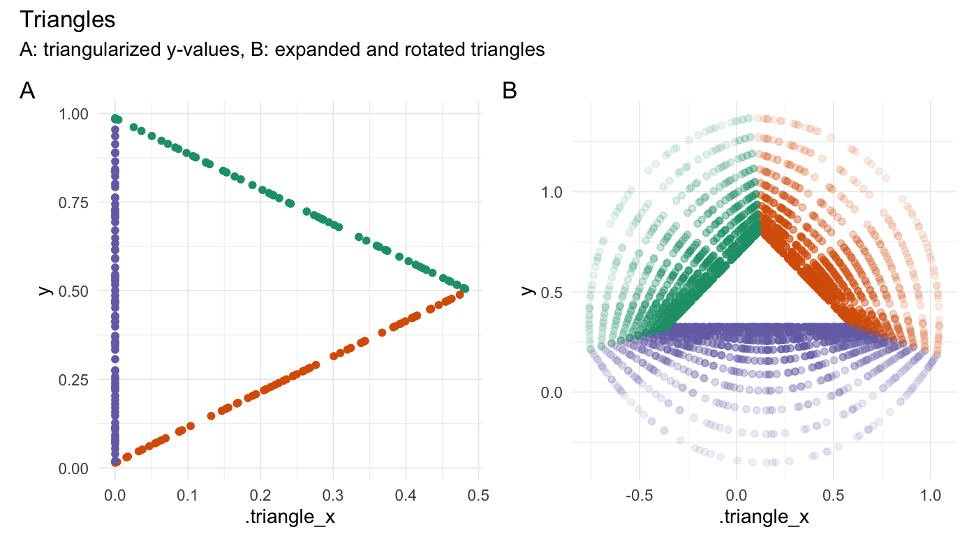
Triangularize points
triangularize(runif(200))
xpectr::set_test_seed(10)

# Create a data frame
df <- data.frame(
  "y" = runif(200)
)

df_tri <- triangularize(df, y_col = "y")

if (has_ggplot){

  ggtri_1 <- df_tri %>%
    ggplot(aes(x = .triangle_x, y = y, color = .edge)) +
    geom_point() +
    theme_minimal(base_line_size = gg_base_line_size) +
    scale_colour_brewer(palette = "Dark2") +
    labs(x = ".triangle_x", y = "y")

}

origin <- centroid(df_tri$.triangle_x, df_tri$y)
df_tri_expanded <- purrr::map_dfr(
  .x = 1:10/10,
  .f = function(mult){
    expand_distances(
      data = df_tri,
      cols = c(".triangle_x", "y"),
      multiplier = mult,
      exponentiate = TRUE,
      add_one_exp = FALSE,
      origin = origin)
  }) %>%
  rotate_2d(
    degrees = 90,
    x_col = ".triangle_x_expanded",
    y_col = "y_expanded",
    suffix = "",
    origin = origin
  )

if (has_ggplot){

  ggtri_2 <- df_tri_expanded %>%
    ggplot(aes(x = .triangle_x_expanded, y = y_expanded,
               color = .edge, alpha = 0.8*.exponent^2)) +
    geom_point() +
    theme_minimal(base_line_size = gg_base_line_size) +
    scale_colour_brewer(palette = "Dark2") +
    labs(x = ".triangle_x", y = "y")

  combined <- (ggtri_1 + ggtri_2) & theme(legend.position = "none")
  combined +
    plot_annotation(title = "Triangles",
                    subtitle = "A: triangularized y-values, B: expanded and rotated triangles",
                    tag_levels = 'A')

}
Generators
Generate clusters
xpectr::set_test_seed(10)
generate_clusters(
  num_rows = 50,
  num_cols = 5,
  num_clusters = 5,
  compactness = 1.6
)
xpectr::set_test_seed(10)

df_clusters <- generate_clusters(
  num_rows = 50, num_cols = 5,
  num_clusters = 5, compactness = 1.6
)

if (has_ggplot){

  df_clusters %>%
    ggplot(
      aes(x = D1, y = D2, color = .cluster)) +
      geom_point() +
      theme_minimal(base_line_size = gg_base_line_size) +
      scale_colour_brewer(palette = "Dark2") +
      labs(x = "D1", y = "D2", color = "Cluster")

}
Utilities
Converters
| Function | Description |
|:----------------------|:----------------------------------------------------------------------|
|radians_to_degrees() |Converts radians to degrees. |
|degrees_to_radians() |Converts degrees to radians. |
Scalers
| Function | Description |
|:----------------------|:----------------------------------------------------------------------|
|min_max_scale() |Scale values to a range. |
|to_unit_length() |Scale vectors to unit length row-wise or column-wise. |
Measuring functions
| Function | Description |
|:----------------------|:----------------------------------------------------------------------|
|distance() |Calculates distance to an origin. |
|angle() |Calculates angle between points and an origin. |
|vector_length() |Calculates vector length/magnitude row-wise or column-wise. |
Helper functions
| Function | Description |
|:----------------------|:----------------------------------------------------------------------|
|create_origin_fn() |Creates function for finding origin coordinates (like centroid()). |
|centroid() |Calculates the mean of each supplied vector/column. |
|most_centered() |Finds coordinates of data point closest to the centroid. |
|is_most_centered() |Indicates whether a data point is the most centered. |
|midrange() |Calculates the midrange of each supplied vector/column. |
|create_n_fn() |Creates function for finding the number of positions to move. |
|median_index() |Calculates median index of each supplied vector. |
|quantile_index() |Calculates quantile of indices for each supplied vector. |
LudvigOlsen/rearrr documentation built on April 12, 2025, 6:37 p.m.
R Package Documentation
Browse R Packages
We want your feedback!
Note that we can't provide technical support on individual packages. You should contact the package authors for that.
if (requireNamespace("knitr", quietly = TRUE)){ knitr::opts_chunk$set( collapse = TRUE, comment = "#>", fig.path = "man/figures/README-", dpi = 92, fig.retina = 2 ) } # Get minimum R requirement dep <- as.vector(read.dcf('DESCRIPTION')[, 'Depends']) rvers <- substring(dep, 7, nchar(dep)-1) # m <- regexpr('R *\\\\(>= \\\\d+.\\\\d+.\\\\d+\\\\)', dep) # rm <- regmatches(dep, m) # rvers <- gsub('.*(\\\\d+.\\\\d+.\\\\d+).*', '\\\\1', dep) # Function for TOC # https://gist.github.com/gadenbuie/c83e078bf8c81b035e32c3fc0cf04ee8
rearrr
Rearrrange Data
Authors: Ludvig R. Olsen ( r-pkgs@ludvigolsen.dk )
![]()
License: MIT
Started: April 2020
![]()
![]()
![]()
Overview
R package for rearranging data by a set of methods.
We distinguish between rearrangers and mutators, where the first reorders the data points and the second changes the values of the data points.
When performing an operation relative to a point in an n-dimensional vector space, we refer to the point as the origin. If we, for instance, wish to rotate our data points around the point at x = 3 and y = 7, those are the coordinates of our origin.
Install
CRAN (when available):
install.packages("rearrr")
Development version:
install.packages("devtools")
devtools::install_github("LudvigOlsen/rearrr")
Rearrangers
| Function | Description |
|:----------------------|:----------------------------------------------------------------------|
|center_max() |Center the highest value with values decreasing around it. |
|center_min() |Center the lowest value with values increasing around it. |
|position_max() |Position the highest value with values decreasing around it. |
|position_min() |Position the lowest value with values increasing around it. |
|pair_extremes() |Arrange as lowest, highest, 2nd lowest, 2nd highest, etc. |
|triplet_extremes() |Arrange as lowest, most middle, highest, 2nd lowest, 2nd most middle, 2nd highest, etc. |
|closest_to() |Order values by shortest distance to an origin. |
|furthest_from() |Order values by longest distance to an origin. |
|rev_windows() |Reverse order window-wise. |
|roll_elements() |Rolls/shifts positions of elements. |
|shuffle_hierarchy() |Shuffle multi-column hierarchy of groups. |
Mutators
| Function | Description | Dimensions |
|:----------------------|:----------------------------------------------------------------------|:-----------|
|rotate_2d(), rotate_3d() |Rotate values around an origin in 2 or 3 dimensions. |2 or 3 |
|swirl_2d(), swirl_3d() |Swirl values around an origin in 2 or 3 dimensions. |2 or 3 |
|shear_2d(), shear_3d() |Shear values around an origin in 2 or 3 dimensions. |2 or 3 |
|expand_distances() |Expand distances to an origin. |n |
|expand_distances_each()|Expand distances to an origin separately for each dimension. |n |
|cluster_groups() |Move data points into clusters around group centroids. |n |
|dim_values() |Dim values of a dimension by the distance to an n-dimensional origin. |n (alters 1)|
|flip_values() |Flip the values around an origin. |n |
|roll_values() |Shifts values and wraps to a range. |n |
|wrap_to_range() |Wraps values to a range. |n |
|transfer_centroids() |Transfer centroids from one data.frame to another. |n |
|apply_transformation_matrix() |Apply transformation matrix to data.frame columns. |n |
Formers
| Function | Description |
|:------------------|:----------------------------------------------------------------------|
|circularize() |Create x-coordinates for y-coordinates so they form a circle. |
|hexagonalize() |Create x-coordinates for y-coordinates so they form a hexagon. |
|square() |Create x-coordinates for y-coordinates so they form a square. |
|triangularize() |Create x-coordinates for y-coordinates so they form a triangle. |
Pipelines
| Class | Description |
|:---------------------|:------------------------------------------------------------------------|
|Pipeline |Chain multiple transformations. |
|GeneratedPipeline |Chain multiple transformations and generate argument values per group. |
|FixedGroupsPipeline |Chain multiple transformations with different argument values per group. |
Generators
| Function | Description |
|:----------------------|:----------------------------------------------------------------------|
|generate_clusters() |Generate n-dimensional clusters. |
Additionally, some functions have *_vec() versions, that take and return a vector.
Note: The available utility functions (like scalers, converters and measuring functions) are listed at the bottom of the readme.
Table of Contents
rearrr:::render_toc("README.Rmd", toc_depth = 4)
Attach packages
Let's see some examples. We start by attaching the necessary packages:
library(rearrr) library(dplyr) xpectr::set_test_seed(1)
library(knitr) # kable() has_tidyr <- require(tidyr) # gather() has_ggplot <- require(ggplot2) # Attach if installed vec <- 1:10 random_sample <- runif(10) orderings <- data.frame( "Position" = as.integer(vec), "center_max" = center_max(vec), "center_min" = center_min(vec), "position_max" = position_max(vec, position = 3), "position_min" = position_min(vec, position = 3), "pair_extremes" = pair_extremes_vec(vec), "rev_windows" = rev_windows_vec(vec, window_size = 3), "closest_to" = closest_to_vec(vec, origin_fn = create_origin_fn(median)), "furthest_from" = furthest_from_vec(vec, origin = 5), "random_sample" = random_sample, "flipped_median" = flip_values_vec(random_sample, origin_fn=create_origin_fn(median)), stringsAsFactors = FALSE ) # Convert to long format for plotting if (has_tidyr){ orderings <- orderings %>% tidyr::gather(key = "Method", value = "Value", 2:(ncol(orderings))) } gg_line_alpha <- .4 gg_base_line_size <- .3
While we can use the functions with data.frames, we showcase many of them with a vector for simplicity.
At times, we use the *_vec() version of a function in order to get the output as a vector instead of a data.frame.
The functions work with grouped data.frames and in magrittr pipelines (%>%).
Rearranger examples
Rearrangers change the order of the data points.
Center min/max
center_max(data = 1:10)
center_min(data = 1:10)
if (has_ggplot && has_tidyr){ # Plot centering methods orderings %>% dplyr::filter(Method %in% c("center_min", "center_max")) %>% ggplot(aes(x = Position, y = Value, color = Method)) + geom_line(alpha = gg_line_alpha) + geom_point() + theme_minimal(base_line_size = gg_base_line_size) + scale_x_continuous(breaks = c(2, 4, 6, 8, 10)) + scale_y_continuous(breaks = c(2, 4, 6, 8, 10)) + scale_colour_brewer(palette = "Dark2") }
Position min/max
position_max(data = 1:10, position = 3)
position_min(data = 1:10, position = 3)
if (has_ggplot && has_tidyr){ # Plot positioning methods orderings %>% dplyr::filter(Method %in% c("position_min", "position_max")) %>% ggplot(aes(x = Position, y = Value, color = Method)) + geom_line(alpha = gg_line_alpha) + geom_point() + theme_minimal(base_line_size = gg_base_line_size) + scale_x_continuous(breaks = c(2, 4, 6, 8, 10)) + scale_y_continuous(breaks = c(2, 4, 6, 8, 10)) + scale_colour_brewer(palette = "Dark2") }
Pair extremes
pair_extremes(data = 1:10)
if (has_ggplot && has_tidyr){ # Plot extreme pairing orderings %>% dplyr::filter(Method == "pair_extremes") %>% ggplot(aes(x = Position, y = Value, color = Method)) + geom_line(alpha = gg_line_alpha) + geom_point() + theme_minimal(base_line_size = gg_base_line_size) + scale_x_continuous(breaks = c(2, 4, 6, 8, 10)) + scale_y_continuous(breaks = c(2, 4, 6, 8, 10)) + scale_colour_brewer(palette = "Dark2") }
Closest to / furthest from
We use the _vec() versions to get the reordered vectors. For data.frames, use closest_to()/furthest_from() instead.
The origin can be passed as either a specific coordinate (here, a value in data) or a function.
closest_to_vec(data = 1:10, origin_fn = create_origin_fn(median))
furthest_from_vec(data = 1:10, origin = 5)
if (has_ggplot && has_tidyr){ # Plot distanced order orderings %>% dplyr::filter(Method %in% c("closest_to", "furthest_from")) %>% ggplot(aes(x = Position, y = Value, color = Method)) + geom_line(alpha = gg_line_alpha) + geom_point() + theme_minimal(base_line_size = gg_base_line_size) + scale_x_continuous(breaks = c(2, 4, 6, 8, 10)) + scale_y_continuous(breaks = c(2, 4, 6, 8, 10)) + scale_colour_brewer(palette = "Dark2") }
Reverse windows
We use the _vec() version to get the reordered vector. For data.frames, use rev_windows() instead.
rev_windows_vec(data = 1:10, window_size = 3)
if (has_ggplot && has_tidyr){ # Plot windowed reversing orderings %>% dplyr::filter(Method == "rev_windows") %>% ggplot(aes(x = Position, y = Value, color = Method)) + geom_line(alpha = gg_line_alpha) + geom_point() + theme_minimal(base_line_size = gg_base_line_size) + scale_x_continuous(breaks = c(2, 4, 6, 8, 10)) + scale_y_continuous(breaks = c(2, 4, 6, 8, 10)) + scale_colour_brewer(palette = "Dark2") }
Shuffle Hierarchy
When having a data.frame with multiple grouping columns, we can shuffle them one column (hierarchical level) at a time:
# Shuffle a given data frame 'df' shuffle_hierarchy(df, group_cols = c("a", "b", "c"))
The columns are shuffled one at a time, as so:
Mutator examples
Mutators change the values of the data points.
Rotate values
2-dimensional rotation:
# Set seed for reproducibility xpectr::set_test_seed(1) # Draw random numbers random_sample <- round(runif(10), digits = 4) random_sample rotate_2d( data = random_sample, degrees = 60, origin_fn = centroid )
rotate_df <- rotate_2d(random_sample, degrees = c(0, 72, 144, 216, 288), origin_fn = centroid) if (has_ggplot){ # Plot rotated values rotate_df %>% ggplot(aes(x = Index_rotated, y = Value_rotated, color = factor(.degrees))) + geom_hline(yintercept = mean(random_sample), size = 0.2, alpha = gg_line_alpha, linetype="dashed") + geom_vline(xintercept = mean(seq_len(length(random_sample))), size = 0.2, alpha = gg_line_alpha, linetype="dashed") + geom_path(alpha = gg_line_alpha) + geom_point() + theme_minimal(base_line_size = gg_base_line_size) + scale_colour_brewer(palette = "Dark2") + labs(x = "Index", y="Value", color="Degrees") }
3-dimensional rotation:
# Set seed set.seed(3) # Create a data frame df <- data.frame( "x" = 1:12, "y" = c(1, 2, 3, 4, 9, 10, 11, 12, 15, 16, 17, 18), "z" = runif(12) ) # Perform rotation rotate_3d( data = df, x_col = "x", y_col = "y", z_col = "z", x_deg = 45, y_deg = 90, z_deg = 135, origin_fn = centroid )
rotate_df <- df %>% rotate_3d(x_col = "x", y_col = "y", z_col = "z", x_deg = c(0, 72, 144, 216, 288), y_deg = c(0, 72, 144, 216, 288), z_deg = c(0, 72, 144, 216, 288), origin_fn = centroid) if (has_ggplot){ # Plot rotated values rotate_df %>% ggplot(aes(x = x_rotated, y = y_rotated, color = .degrees_str, alpha = z_rotated)) + geom_vline(xintercept = mean(df$x), size = 0.2, alpha = .4, linetype="dashed") + geom_hline(yintercept = mean(df$y), size = 0.2, alpha = .4, linetype="dashed") + geom_path(alpha = gg_line_alpha) + geom_point() + theme_minimal(base_line_size = gg_base_line_size) + scale_colour_brewer(palette = "Dark2") + labs(x = "x", y = "y", color = "degrees", alpha = "z (opacity)") }
Swirl values
2-dimensional swirling:
# Rotate values swirl_2d(data = rep(1, 50), radius = 95, origin = c(0, 0))
# Swirl around the centroid df_swirled <- swirl_2d( data = rep(1, 50), radius = c(95, 96, 97, 98, 99, 100), origin_fn = centroid, suffix = "", scale_fn = function(x) { x ^ 1.6 } ) orig <- df_swirled$.origin[[1]] if (has_ggplot){ # Plot swirls ggswirl1 <- df_swirled %>% ggplot(aes(x = Index, y = Value, color = factor(.radius))) + geom_point() + theme_minimal(base_line_size = gg_base_line_size) + scale_colour_brewer(palette = "Dark2") + labs(x = "x", y = "y", color = ".radius") } df_swirled <- df_swirled %>% rotate_2d(degrees = (1:36) * 10, x_col = "Index", y_col = "Value", suffix = "", origin = orig) if (has_ggplot){ # Plot rotated swirls ggswirl2 <- df_swirled %>% ggplot(aes(x = Index, y = Value, color = factor(.radius))) + geom_point() + theme_minimal(base_line_size = gg_base_line_size) + scale_colour_brewer(palette = "Dark2") + labs(x = "x", y = "y", color = ".radius") } # Expand values ^2 df_swirled <- df_swirled %>% expand_distances( cols = c("Index", "Value"), multiplier = 2, exponentiate = T, origin = orig, suffix = "") if (has_ggplot){ # Plot expanded swirls ggswirl3 <- df_swirled %>% ggplot(aes(x = Index, y = Value, color = factor(.radius))) + geom_point() + theme_minimal(base_line_size = gg_base_line_size) + scale_colour_brewer(palette = "Dark2") + labs(x = "x", y = "y", color = ".radius") } # Dim values df_swirled <- df_swirled %>% mutate(o = 1) %>% dim_values(cols = c("Index", "Value", "o"), origin = c(orig, 1), suffix = "") if (has_ggplot){ # Plot rotated swirls ggswirl4 <- df_swirled %>% ggplot(aes(x = Index, y = Value, alpha = o, color = factor(.radius))) + geom_point() + theme_minimal(base_line_size = gg_base_line_size) + scale_colour_brewer(palette = "Dark2") + labs(x = "x", y = "y", color = ".radius", alpha = "opacity (for D)") combined <- (ggswirl1 + ggswirl2) / (ggswirl3 + ggswirl4) & theme(legend.position = "bottom") combined <- combined + plot_layout(guides = "collect") combined + plot_annotation(title = "2d swirls with rotation, expansion and dimming", subtitle = "A: 2d swirls, B: Rotated A, C: Expanded B, D: Dimmed C", caption = "Distances in A are scaled by d^1.6", tag_levels = 'A') }
3-dimensional swirling:
# Set seed set.seed(4) # Create a data frame df <- data.frame( "x" = 1:50, "y" = 1:50, "z" = 1:50, "r1" = runif(50), "r2" = runif(50) * 35, "o" = 1, "g" = rep(1:5, each = 10) ) # They see me swiiirling swirl_3d( data = df, x_radius = 45, x_col = "x", y_col = "y", z_col = "z", origin = c(0, 0, 0), keep_original = FALSE )
# 1st plot df_swirled <- swirl_3d( data = df, x_col = "x", y_col = "y", z_col = "z", x_radius = c(100, 0, 0), y_radius = c(0, 100, 0), z_radius = c(0, 0, 100), origin_fn = centroid ) if (has_ggplot){ ggswirl_3d_1 <- df_swirled %>% ggplot(aes(x = x_swirled, y = y_swirled, color = .radius_str, alpha = z_swirled)) + geom_path(alpha = gg_line_alpha) + geom_point() + theme_minimal(base_line_size = gg_base_line_size) + scale_colour_brewer(palette = "Dark2") + labs(x = "x", y = "y", color = "radius", alpha = "z (opacity)") } # 2nd plot df_swirled <- swirl_3d( data = df, x_col = "x", y_col = "y", z_col = "z", x_radius = c(50, 0, 0), y_radius = c(0, 50, 0), z_radius = c(0, 0, 50), origin_fn = centroid ) if (has_ggplot){ ggswirl_3d_2 <- df_swirled %>% ggplot(aes(x = x_swirled, y = y_swirled, color = .radius_str, alpha = z_swirled)) + geom_path(alpha = gg_line_alpha) + geom_point() + theme_minimal(base_line_size = gg_base_line_size) + scale_colour_brewer(palette = "Dark2") + labs(x = "x", y = "y", color = "radius", alpha = "z (opacity)") } # 3rd plot df_swirled <- swirl_3d( data = df, x_col = "x", y_col = "y", z_col = "z", x_radius = c(25, 50, 25, 25), y_radius = c(50, 75, 100, 25), z_radius = c(75, 25, 25, 25), origin_fn = centroid, scale_fn = function(x) { x^0.81 } ) if (has_ggplot){ ggswirl_3d_3 <- df_swirled %>% ggplot(aes(x = x_swirled, y = y_swirled, color = .radius_str, alpha = z_swirled)) + geom_path(alpha = gg_line_alpha) + geom_point() + theme_minimal(base_line_size = gg_base_line_size) + scale_colour_brewer(palette = "Dark2") + labs(x = "x", y = "y", color = "radius", alpha = "z (opacity)") } # 4th plot df_swirled <- swirl_3d( data = df, x_col = "r1", y_col = "r2", z_col = "o", x_radius = c(0, 0, 0, 0), y_radius = c(0, 30, 60, 90), z_radius = c(10, 10, 10, 10), origin_fn = centroid ) # Not let's rotate it every 10 degrees df_rotated <- df_swirled %>% rotate_3d( x_col = "r1_swirled", y_col = "r2_swirled", z_col = "o_swirled", x_deg = rep(0, 36), y_deg = rep(0, 36), z_deg = (1:36) * 10, suffix = "", origin = df_swirled$.origin[[1]]) if (has_ggplot){ ggswirl_3d_4 <- df_rotated %>% ggplot(aes(x = r1_swirled, y = r2_swirled, color = .degrees_str, alpha = o_swirled)) + geom_point(show.legend = FALSE) + theme_minimal(base_line_size = gg_base_line_size) + # scale_colour_brewer(palette = "Dark2") + labs(x = "r1", y = "r2", color = "radius", alpha = "o (opacity)") combined <- (ggswirl_3d_1 + ggswirl_3d_2) / (ggswirl_3d_3 + ggswirl_3d_4) & theme(legend.position = "none") # combined <- combined + plot_layout(guides = "collect") combined + plot_annotation(title = "3d swirls", subtitle = "ABC: 3d swirls, D: rotated 3d swirls", caption = "Distances in C are scaled by d^0.81", tag_levels = 'A') }
Expand distances
# 1d expansion expand_distances( data = random_sample, multiplier = 3, origin_fn = centroid, exponentiate = TRUE )
2d expansion:
xpectr::set_test_seed(36) random_x <- runif(10) random_y <- runif(10) expand_df <- purrr::map_dfr( .x = c(1, 2, 3, 4, 5), .f = function(exponent) { expand_distances( data.frame("x" = random_x, "y" = random_y), cols = c("x", "y"), multiplier = exponent, origin_fn = centroid, exponentiate = TRUE ) } ) if (has_ggplot){ # Plot rotated values expand_df %>% ggplot(aes(x = x_expanded, y = y_expanded, color = factor(.exponent))) + geom_hline(yintercept = mean(random_y), size = 0.2, alpha = gg_line_alpha, linetype="dashed") + geom_vline(xintercept = mean(random_x), size = 0.2, alpha = gg_line_alpha, linetype="dashed") + geom_path(alpha = gg_line_alpha) + geom_point() + theme_minimal(base_line_size = gg_base_line_size) + scale_colour_brewer(palette = "Dark2") + labs(x = "x", y="y", color="Exponent") } xpectr::set_test_seed(36) # for next section
Expand differently in each axis:
# Expand x-axis and contract y-axis expand_distances_each( data.frame("x" = runif(10), "y" = runif(10)), cols = c("x", "y"), multipliers = c(7, 0.5), origin_fn = centroid )
rand_df <- data.frame("x" = random_x, "y" = random_y) expand_df <- purrr::map2_dfr( .x = c(7, 1), .y = c(0.5, 1), .f = function(m1, m2) { expand_distances_each( rand_df, cols = c("x", "y"), multipliers = c(m1, m2), origin_fn = centroid ) } ) if (has_ggplot){ # Plot rotated values expand_df %>% ggplot(aes(x = x_expanded, y = y_expanded, color = factor(.multipliers_str))) + geom_hline(yintercept = mean(random_y), size = 0.2, alpha = gg_line_alpha, linetype = "dashed") + geom_vline(xintercept = mean(random_x), size = 0.2, alpha = gg_line_alpha, linetype = "dashed") + geom_path(alpha = gg_line_alpha) + geom_point() + theme_minimal(base_line_size = gg_base_line_size) + scale_colour_brewer(palette = "Dark2") + labs(x = "x", y = "y", color = "Multiplier") }
Cluster groups
# Set seed for reproducibility xpectr::set_test_seed(3) # Create data frame with random data and a grouping variable df <- data.frame( "x" = runif(50), "y" = runif(50), "g" = rep(c(1, 2, 3, 4, 5), each = 10) ) cluster_groups( data = df, cols = c("x", "y"), group_col = "g" )
df_clustered <- cluster_groups(df, cols = c("x", "y"), group_col = "g") if (has_ggplot){ ggplot(df_clustered, aes(x = x_clustered, y = y_clustered, color = factor(g))) + # Original data geom_point(aes(x = x, y = y), alpha = 0.3, size = 0.8) + # Clustered data geom_point() + theme_minimal(base_line_size = gg_base_line_size) + scale_colour_brewer(palette = "Dark2") + labs(x = "x", y = "y", color = "g", caption = "Semi-transparent points are the original data points.") } df_clustered <- df_clustered %>% dplyr::select(x_clustered, y_clustered, g)
Dim values
# Add a column with 1s df_clustered$o <- 1 # Dim the "o" column based on the data point's distance # to the most central point in the cluster df_clustered %>% dplyr::group_by(g) %>% dim_values( cols = c("x_clustered", "y_clustered"), dim_col = "o", origin_fn = most_centered )
df_dimmed <- df_clustered %>% dplyr::group_by(g) %>% dim_values(cols = c("x_clustered", "y_clustered", "o"), origin_fn = most_centered) if (has_ggplot){ ggplot(df_dimmed, aes(x = x_clustered, y = y_clustered, alpha = o_dimmed, color = factor(g))) + geom_point() + theme_minimal(base_line_size = gg_base_line_size) + scale_colour_brewer(palette = "Dark2") + labs(x = "x", y = "y", color = "g", alpha = "o_dimmed") }
Flip values
# The median value to flip around median(random_sample) # Flip the random numbers around the median flip_values( data = random_sample, origin_fn = create_origin_fn(median) )
if (has_ggplot && has_tidyr){ # Plot flipped values orderings %>% dplyr::filter(Method %in% c("random_sample", "flipped_median")) %>% ggplot(aes(x = Position, y = Value, color = Method)) + geom_line(alpha = gg_line_alpha) + geom_point() + theme_minimal(base_line_size = gg_base_line_size) + scale_x_continuous(breaks = c(2, 4, 6, 8, 10)) + scale_colour_brewer(palette = "Dark2") }
Forming examples
Circularize points
circularize(runif(200))
xpectr::set_test_seed(10) # Create a data frame df <- data.frame( "y" = runif(200) ) df_circ <- circularize(df, y_col = "y") if (has_ggplot){ ggcirc_1 <- df_circ %>% ggplot(aes(x = .circle_x, y = y, color = .degrees)) + geom_point() + theme_minimal(base_line_size = gg_base_line_size) + scale_colour_distiller(palette = "Dark2") + labs(x = ".circle_x", y = "y") } df_circ_expanded <- purrr::map_dfr( .x = 1:10/10, .f = function(mult){ expand_distances( data = df_circ, cols = c(".circle_x", "y"), multiplier = mult, origin_fn = centroid) }) if (has_ggplot){ ggcirc_2 <- df_circ_expanded %>% ggplot(aes(x = .circle_x_expanded, y = y_expanded, color = .degrees, alpha = 0.8*.multiplier^2)) + geom_point(aes(size = 0.8*.multiplier^2)) + theme_minimal(base_line_size = gg_base_line_size) + scale_colour_distiller(palette = "Dark2") + labs(x = ".circle_x", y = "y") combined <- (ggcirc_1 + ggcirc_2) & theme(legend.position = "none") combined + plot_annotation(title = "Circles", subtitle = "A: circularized y-values, B: contracted circles", tag_levels = 'A') }
Hexagonalize points
hexagonalize(runif(200))
xpectr::set_test_seed(10) # Create a data frame df <- data.frame( "y" = runif(200) ) df_hex <- hexagonalize(df, y_col = "y") if (has_ggplot){ gghex_1 <- df_hex %>% ggplot(aes(x = .hexagon_x, y = y, color = .edge)) + geom_point() + theme_minimal(base_line_size = gg_base_line_size) + scale_colour_brewer(palette = "Dark2") + labs(x = ".hexagon_x", y = "y") } df_hex_expanded <- purrr::map_dfr( .x = 1:5/10*2, .f = function(mult){ expand_distances( data = df_hex, cols = c(".hexagon_x", "y"), multiplier = mult, exponentiate = TRUE, origin_fn = centroid) }) if (has_ggplot){ gghex_2 <- df_hex_expanded %>% ggplot(aes(x = .hexagon_x_expanded, y = y_expanded, color = .edge, alpha = 0.8*.exponent^2)) + geom_point(aes(size = 0.8*.exponent^2)) + theme_minimal(base_line_size = gg_base_line_size) + scale_colour_brewer(palette = "Dark2") + labs(x = ".hexagon_x", y = "y") combined <- (gghex_1 + gghex_2) & theme(legend.position = "none") combined + plot_annotation(title = "Hexagons", subtitle = "A: hexagonalized y-values, B: contracted hexagons", tag_levels = 'A') }
Square points
square(runif(200))
df_sq <- square(df, y_col = "y") if (has_ggplot){ ggsq_1 <- df_sq %>% ggplot(aes(x = .square_x, y = y, color = .edge)) + geom_point() + theme_minimal(base_line_size = gg_base_line_size) + scale_colour_brewer(palette = "Dark2") + labs(x = ".square_x", y = "y") } df_sq_expanded <- purrr::map_dfr( .x = c(1, 0.75, 0.5, 0.25, 0.125), .f = function(mult){ expand_distances( data = df_sq, cols = c(".square_x", "y"), multiplier = mult, origin_fn = centroid) }) %>% swirl_2d( radius = 0.3, x_col = ".square_x_expanded", y_col = "y_expanded", origin_fn = centroid, suffix = "", origin_col_name = NULL ) if (has_ggplot){ ggsq_2 <- df_sq_expanded %>% ggplot(aes(x = .square_x_expanded, y = y_expanded, color = .edge, alpha = 0.8*.multiplier^2)) + geom_point(aes(size = 0.8*.multiplier^2)) + theme_minimal(base_line_size = gg_base_line_size) + scale_colour_brewer(palette = "Dark2") + labs(x = ".square_x", y = "y") combined <- (ggsq_1 + ggsq_2) & theme(legend.position = "none") combined + plot_annotation(title = "Squares", subtitle = "A: squared y-values, B: contracted and swirled squares", tag_levels = 'A') }
Triangularize points
triangularize(runif(200))
xpectr::set_test_seed(10) # Create a data frame df <- data.frame( "y" = runif(200) ) df_tri <- triangularize(df, y_col = "y") if (has_ggplot){ ggtri_1 <- df_tri %>% ggplot(aes(x = .triangle_x, y = y, color = .edge)) + geom_point() + theme_minimal(base_line_size = gg_base_line_size) + scale_colour_brewer(palette = "Dark2") + labs(x = ".triangle_x", y = "y") } origin <- centroid(df_tri$.triangle_x, df_tri$y) df_tri_expanded <- purrr::map_dfr( .x = 1:10/10, .f = function(mult){ expand_distances( data = df_tri, cols = c(".triangle_x", "y"), multiplier = mult, exponentiate = TRUE, add_one_exp = FALSE, origin = origin) }) %>% rotate_2d( degrees = 90, x_col = ".triangle_x_expanded", y_col = "y_expanded", suffix = "", origin = origin ) if (has_ggplot){ ggtri_2 <- df_tri_expanded %>% ggplot(aes(x = .triangle_x_expanded, y = y_expanded, color = .edge, alpha = 0.8*.exponent^2)) + geom_point() + theme_minimal(base_line_size = gg_base_line_size) + scale_colour_brewer(palette = "Dark2") + labs(x = ".triangle_x", y = "y") combined <- (ggtri_1 + ggtri_2) & theme(legend.position = "none") combined + plot_annotation(title = "Triangles", subtitle = "A: triangularized y-values, B: expanded and rotated triangles", tag_levels = 'A') }
Generators
Generate clusters
xpectr::set_test_seed(10)
generate_clusters( num_rows = 50, num_cols = 5, num_clusters = 5, compactness = 1.6 )
xpectr::set_test_seed(10) df_clusters <- generate_clusters( num_rows = 50, num_cols = 5, num_clusters = 5, compactness = 1.6 ) if (has_ggplot){ df_clusters %>% ggplot( aes(x = D1, y = D2, color = .cluster)) + geom_point() + theme_minimal(base_line_size = gg_base_line_size) + scale_colour_brewer(palette = "Dark2") + labs(x = "D1", y = "D2", color = "Cluster") }
Utilities
Converters
| Function | Description |
|:----------------------|:----------------------------------------------------------------------|
|radians_to_degrees() |Converts radians to degrees. |
|degrees_to_radians() |Converts degrees to radians. |
Scalers
| Function | Description |
|:----------------------|:----------------------------------------------------------------------|
|min_max_scale() |Scale values to a range. |
|to_unit_length() |Scale vectors to unit length row-wise or column-wise. |
Measuring functions
| Function | Description |
|:----------------------|:----------------------------------------------------------------------|
|distance() |Calculates distance to an origin. |
|angle() |Calculates angle between points and an origin. |
|vector_length() |Calculates vector length/magnitude row-wise or column-wise. |
Helper functions
| Function | Description |
|:----------------------|:----------------------------------------------------------------------|
|create_origin_fn() |Creates function for finding origin coordinates (like centroid()). |
|centroid() |Calculates the mean of each supplied vector/column. |
|most_centered() |Finds coordinates of data point closest to the centroid. |
|is_most_centered() |Indicates whether a data point is the most centered. |
|midrange() |Calculates the midrange of each supplied vector/column. |
|create_n_fn() |Creates function for finding the number of positions to move. |
|median_index() |Calculates median index of each supplied vector. |
|quantile_index() |Calculates quantile of indices for each supplied vector. |
R Package Documentation
Browse R Packages
We want your feedback!
Note that we can't provide technical support on individual packages. You should contact the package authors for that.
Embedding an R snippet on your website
Add the following code to your website.
For more information on customizing the embed code, read Embedding Snippets.