README.md
In MatteoTiratelli/SparsePanelMatch: SparsePanelMatch
SparsePanelMatch
Applies Imai, Kim & Wang (2018) "Matching Methods for Causal Inference with Time-Series Cross-Sectional Data" to sparse panel data where observations are irregular and unbalanced with many missing values.
Procedure:
1. Match each treated observation (unit-time) to untreated observations occurring within a user-defined time window
2. Limit that matched set to control observations with exactly the same treatment history over the last n observations
3. Within that matched set, refine further or weight using Propensity Scores, Covariate Balancing Propensity Scores or Mahalanobis distance
4. Calculate a Difference-in-Difference estimator across the matched sets (with bootstrapped standard errors)
Installation
devtools::install_github("https://github.com/MatteoTiratelli/SparsePanelMatch")
Motivating example
Imai, Kim & Wang (2018) have developed a matching procedure to facilitate causal inference with time-series cross-sectional data. Although their approach is more general, their software package (PanelMatch) only works with regular panel data where there are repeated observations of each unit at identical and equally spaced moments in time. A canonical example might be repeated observations of countries each year.
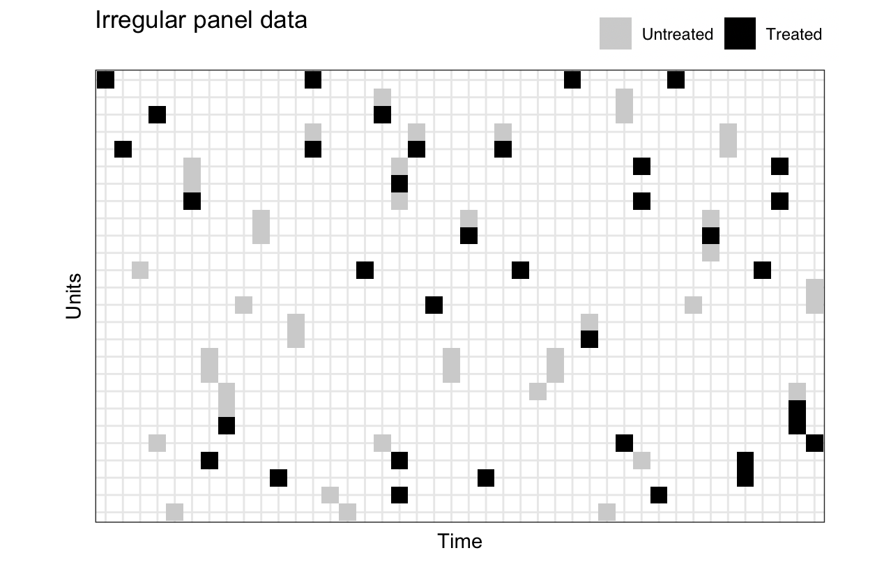
There are times, however, when observations are irregular by design. For example, elections rarely coincide across countries. Data of this sort might look like the graph below, with irregular observations and much missing data.
Matching procedure
Example code:
matches  <- Sparse_PanelMatch(data = CMP, time = "date", unit = "party",
                  treatment = "wasingov", outcome = "sdper103",
                  treatment_lags = 3, outcome_leads = 2,
                  time_window_in_months = 60, match_missing = TRUE,
                  covs = c("pervote", "lag_sd_rile"), qoi = "att",
                  refinement_method = "CBPS.match", size_match = 5,
                  use_diagonal_covmat = TRUE)
Exact matching:
1. The time_window_in_months argument matches each treated observation (unit-time) with untreated observations occurring within a user-defined time window (this is the only significant difference to the original method, where it is assumed that the panel data is well-ordered and regular, meaning that each observation is matched with every other observation at that year/month/date).
2. Within that matched set, the treatment_lags argument then selects control observations with exactly the same treatment history over the last n observations (e.g. over the last three election cycles).
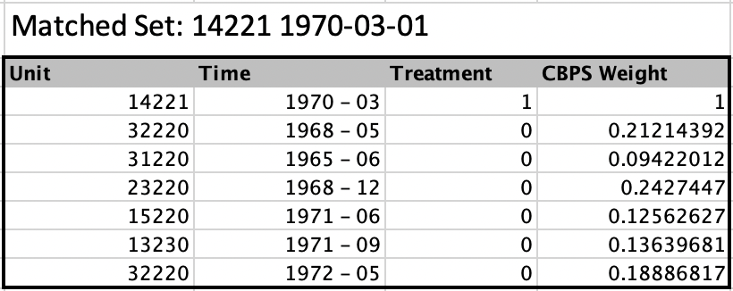
In the example below, we match observations which (a) occurred within a 5 period window of the treated observation, and (b) have exactly the same treatment history over the previous 2 observations.

Refinement:
- After this exact matching procedure, the
refinement_method argument then allows users to further improve covariate balance by calculating Propensity Scores, Covariate Balancing Propensity Scores and Mahalanobis distances. These can be used to (a) create weights for each control observation (ps.weight, CBPS.weight), or (b) to limit the size of the set of control observations (mahalanobis, ps.match, CBPS.match - all must be used with size_match). Covariates are specified using covs. For details see Imai, Kim & Wang (2018).
Estimation procedure
Example code:
estimates <- Sparse_PanelEstimate(data = matches, n_iterations = 1000, alpha = 0.05)
plot(estimates)
- The package then allows users to calculate the Average Treatment effect on Treated/Control via a Difference-in-Difference estimator: within each matched set, we compare the difference in the treated unit with the (weighted) mean difference in control units. In pseudo-code:
DiD = (Yt - Yt-1) - mean(Y't - Y't-1), where Yt is the outcome variable for the treated observation at time t, and Y't is the outcome variable for a control observation at time t. NB Users must specify ATT or ATC in the matching stage via qoi = c("att", "atc").
- These can be calculated for n leads of the outcome variable (specified via
outcome_leads), allowing users to observe the long run impact of the treatment. In that case, for each lead L, we calculate the difference between the outcome at time t+L and the outcome at t-1 for all treated and control observations.
- The final estimand is the mean of the Difference-in-Difference scores across all matched sets. A separate estimand is computed for each lead.
- Standard errors are then calculated by block bootstrapping (resampling across units), and the package allows users to generate both standard percentile and bias-corrected confidence intervals.

MatteoTiratelli/SparsePanelMatch documentation built on March 9, 2023, 3:45 p.m.
R Package Documentation
Browse R Packages
We want your feedback!
Note that we can't provide technical support on individual packages. You should contact the package authors for that.
SparsePanelMatch
Applies Imai, Kim & Wang (2018) "Matching Methods for Causal Inference with Time-Series Cross-Sectional Data" to sparse panel data where observations are irregular and unbalanced with many missing values.
Procedure: 1. Match each treated observation (unit-time) to untreated observations occurring within a user-defined time window 2. Limit that matched set to control observations with exactly the same treatment history over the last n observations 3. Within that matched set, refine further or weight using Propensity Scores, Covariate Balancing Propensity Scores or Mahalanobis distance 4. Calculate a Difference-in-Difference estimator across the matched sets (with bootstrapped standard errors)
Installation
devtools::install_github("https://github.com/MatteoTiratelli/SparsePanelMatch")
Motivating example
Imai, Kim & Wang (2018) have developed a matching procedure to facilitate causal inference with time-series cross-sectional data. Although their approach is more general, their software package (PanelMatch) only works with regular panel data where there are repeated observations of each unit at identical and equally spaced moments in time. A canonical example might be repeated observations of countries each year.
There are times, however, when observations are irregular by design. For example, elections rarely coincide across countries. Data of this sort might look like the graph below, with irregular observations and much missing data.
Matching procedure
Example code:
matches <- Sparse_PanelMatch(data = CMP, time = "date", unit = "party",
treatment = "wasingov", outcome = "sdper103",
treatment_lags = 3, outcome_leads = 2,
time_window_in_months = 60, match_missing = TRUE,
covs = c("pervote", "lag_sd_rile"), qoi = "att",
refinement_method = "CBPS.match", size_match = 5,
use_diagonal_covmat = TRUE)
Exact matching:
1. The time_window_in_months argument matches each treated observation (unit-time) with untreated observations occurring within a user-defined time window (this is the only significant difference to the original method, where it is assumed that the panel data is well-ordered and regular, meaning that each observation is matched with every other observation at that year/month/date).
2. Within that matched set, the treatment_lags argument then selects control observations with exactly the same treatment history over the last n observations (e.g. over the last three election cycles).
In the example below, we match observations which (a) occurred within a 5 period window of the treated observation, and (b) have exactly the same treatment history over the previous 2 observations.
Refinement:
- After this exact matching procedure, the
refinement_methodargument then allows users to further improve covariate balance by calculating Propensity Scores, Covariate Balancing Propensity Scores and Mahalanobis distances. These can be used to (a) create weights for each control observation (ps.weight,CBPS.weight), or (b) to limit the size of the set of control observations (mahalanobis,ps.match,CBPS.match- all must be used withsize_match). Covariates are specified usingcovs. For details see Imai, Kim & Wang (2018).
Estimation procedure
Example code:
estimates <- Sparse_PanelEstimate(data = matches, n_iterations = 1000, alpha = 0.05)
plot(estimates)
- The package then allows users to calculate the Average Treatment effect on Treated/Control via a Difference-in-Difference estimator: within each matched set, we compare the difference in the treated unit with the (weighted) mean difference in control units. In pseudo-code:
DiD = (Yt - Yt-1) - mean(Y't - Y't-1), whereYtis the outcome variable for the treated observation at timet, andY'tis the outcome variable for a control observation at timet. NB Users must specify ATT or ATC in the matching stage viaqoi = c("att", "atc"). - These can be calculated for n leads of the outcome variable (specified via
outcome_leads), allowing users to observe the long run impact of the treatment. In that case, for each leadL, we calculate the difference between the outcome at timet+Land the outcome att-1for all treated and control observations. - The final estimand is the mean of the Difference-in-Difference scores across all matched sets. A separate estimand is computed for each lead.
- Standard errors are then calculated by block bootstrapping (resampling across units), and the package allows users to generate both standard percentile and bias-corrected confidence intervals.
R Package Documentation
Browse R Packages
We want your feedback!
Note that we can't provide technical support on individual packages. You should contact the package authors for that.
Embedding an R snippet on your website
Add the following code to your website.
For more information on customizing the embed code, read Embedding Snippets.