In MikkoVihtakari/ggOceanMaps: Plot Data on Oceanographic Maps using 'ggplot2'

library(knitr)
knitr::opts_chunk$set(collapse = TRUE, 
                      message = FALSE, 
                      warning = FALSE, 
                      eval = FALSE,
                      comment = "#>"
)

library(ggOceanMaps)

General

In addition to the standard maps, the ggOceanMaps package contains a possibility to plot premade detailed shapefiles within limited regions the package author has needed in his work. The detailed shapefiles are stored in the ggOceanMapsLargeData repository and downloaded as needed. Available shapefiles can be viewed using the shapefile_list() function.

shapefile_list("all")

Plotting shapefiles from the list is done as for any other shapes. Note that the projection of the shapefiles varies.

basemap(shapefiles = "BarentsSea", bathymetry = TRUE)

The detailed shapefiles can be large. Use the standard basemap data sources to find the limits for your map before you make detailed plots. Exporting to a file is advised over plotting into the plot window. Note that the detailed shapefile approach generally does not work for large areas. The solution is sub-optimal and a possibility of plotting raster from WMS is under work.

Standard map {#standard-maps}

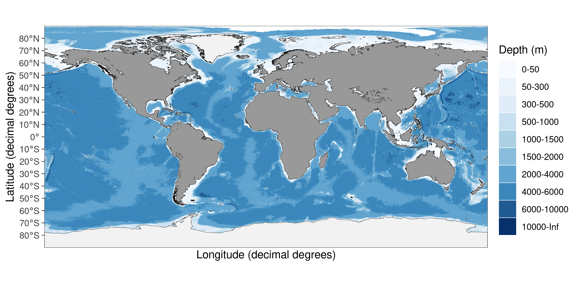
The default

The default map coming with ggOceanMaps uses decimal degrees and Natural Earth Data 1:10m Physical Vectors with the Land and Minor Island datasets combined. The map is transformed to other polar stereographic projections based on limits used in the map.

basemap("DecimalDegree", bathymetry = TRUE, glaciers = TRUE)

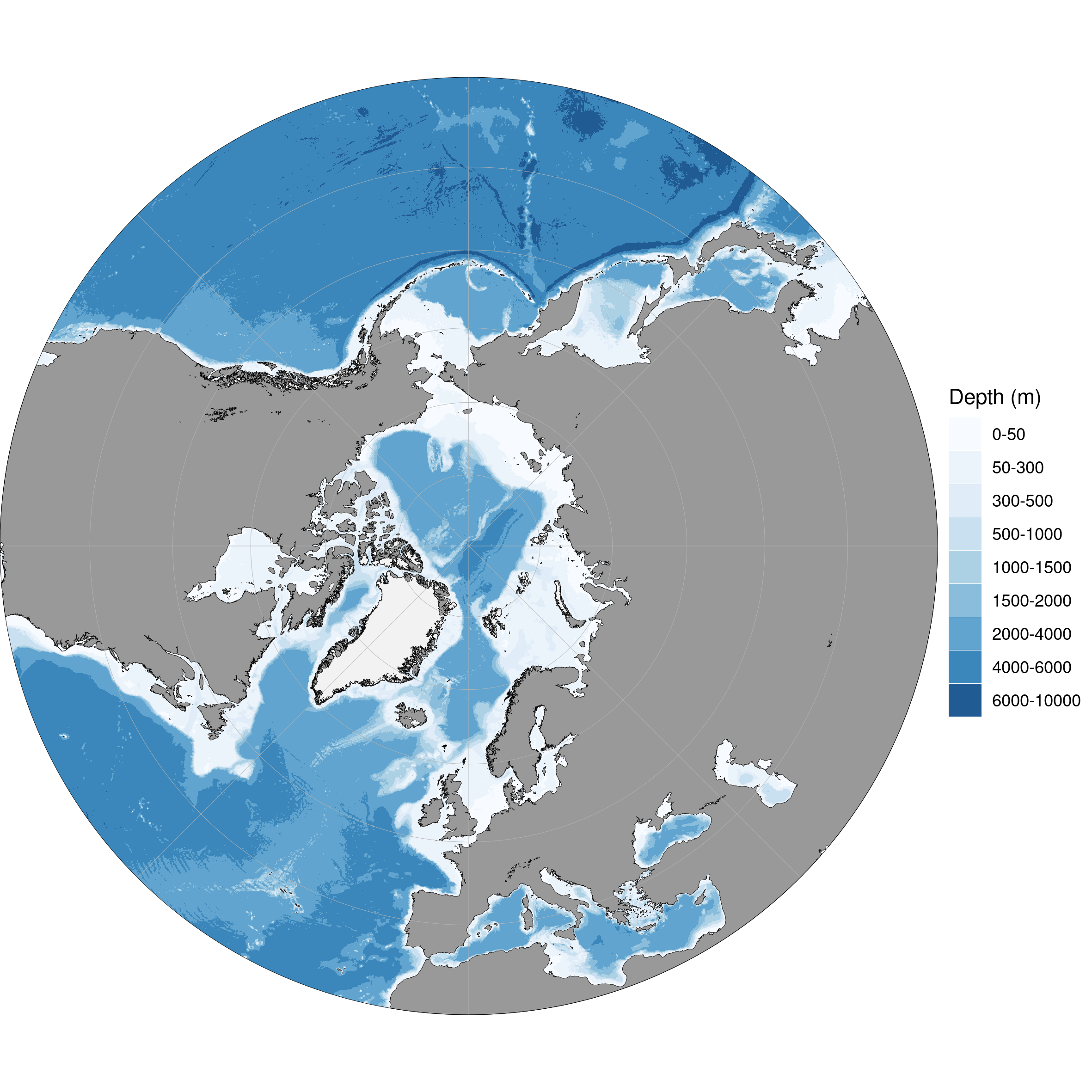
Arctic Stereographic

Standard maps requiring the ggOceanMapsData package are selected automatically based on limits used in the map. You can also use the shapefiles argument or the x argument as a shortcut to specifically plot these maps (the shortcut requires ggOceanMaps >=1.3.1). Since partial matching is used, you do not need write out the entire name. Only "Arctic" will do for the Arctic stereographic map, for instance.

basemap("ArcticStereographic", bathymetry = TRUE, glaciers = TRUE)

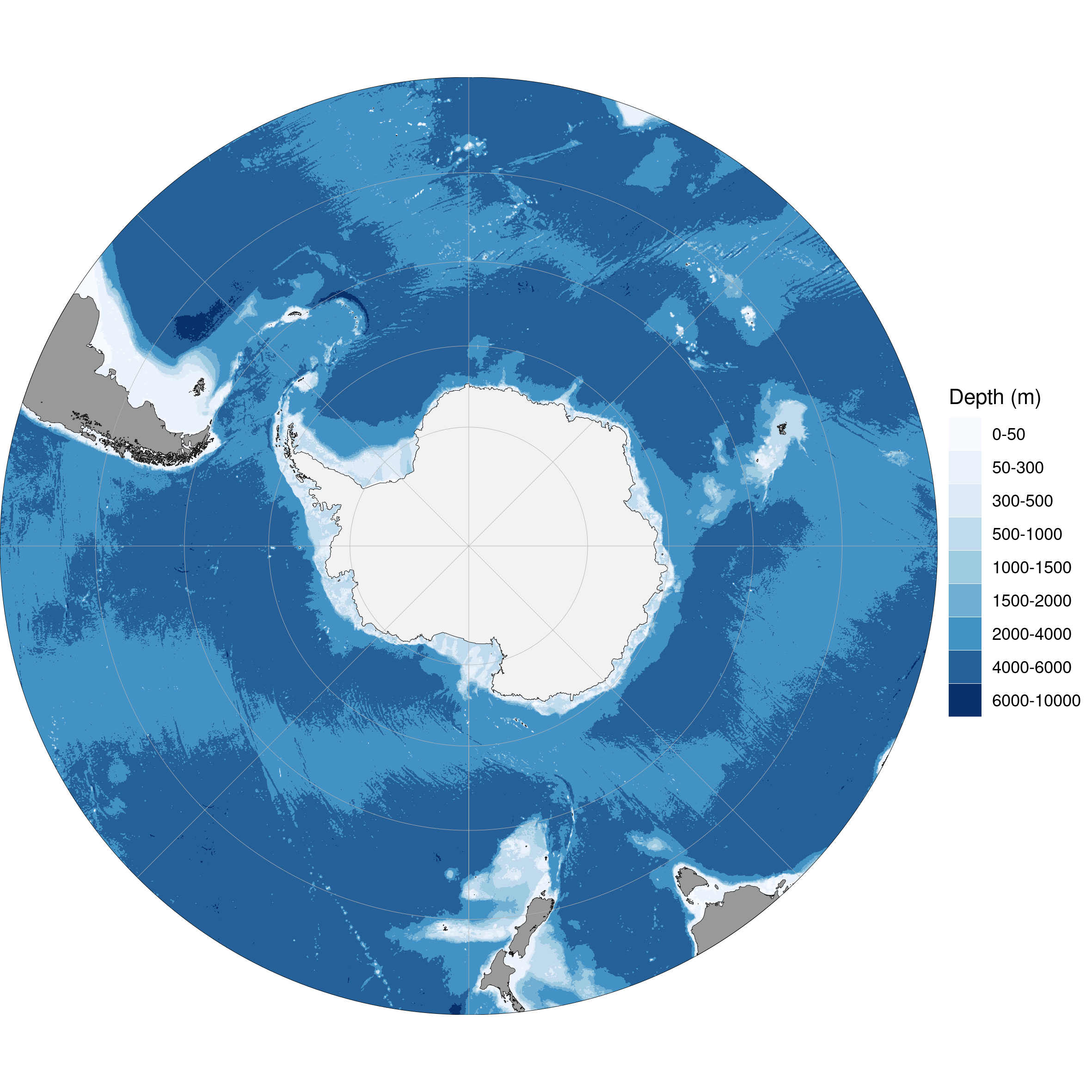
Antarctic Stereographic

basemap("AntarcticStereographic", bathymetry = TRUE, glaciers = TRUE)

Decimal degree

The detailed shapefiles for time being are:

GEBCO based maps

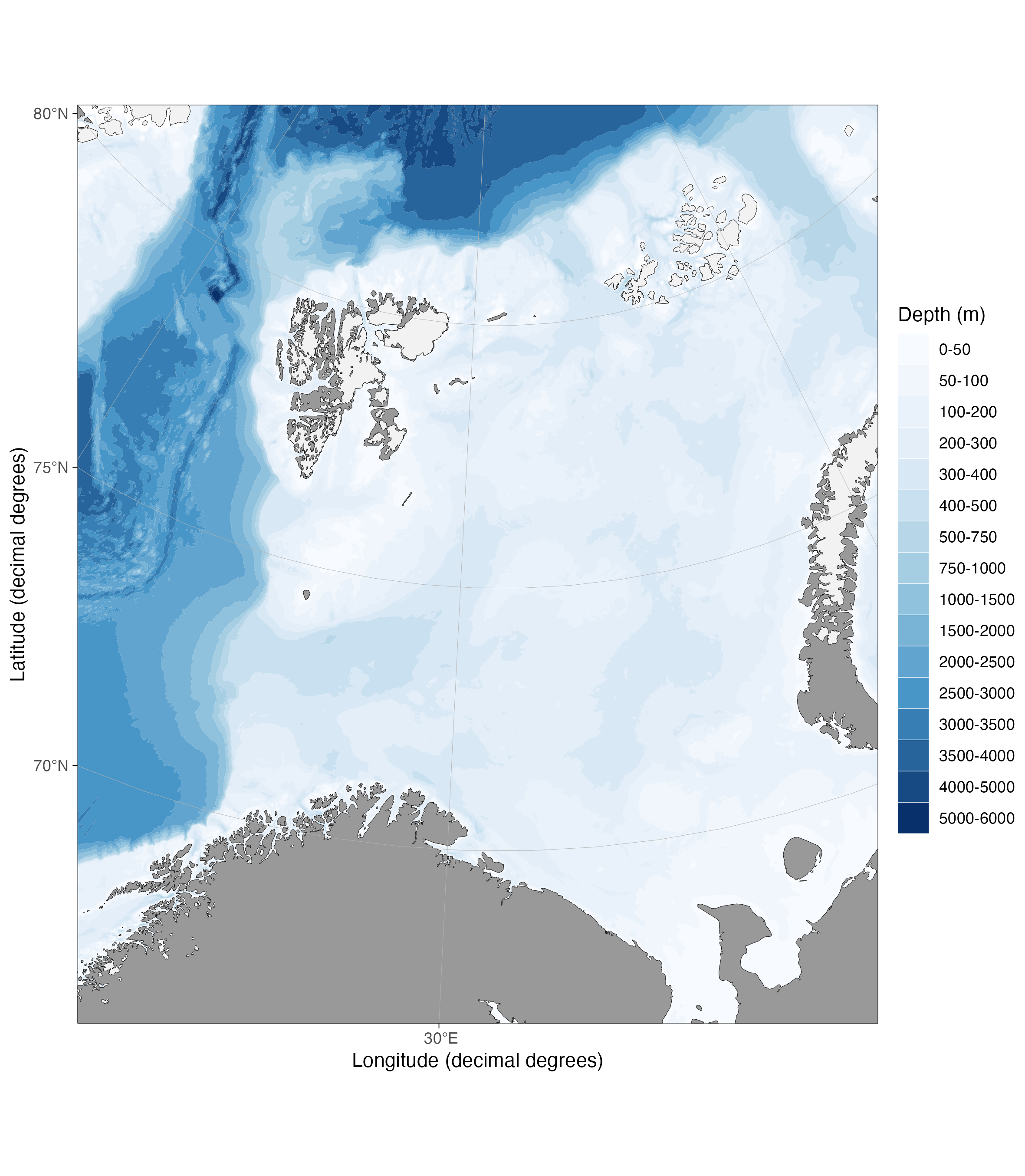
Barents Sea

The Barents Sea and surroundings vectorized from the GEBCO grid. A subset of IBCAO and GEBCO datasets. Use this one for speed when you can. Replace by IBCAO when your ROI is exceeding the limits of this one.

basemap("BarentsSea", bathymetry = TRUE, glaciers = TRUE)

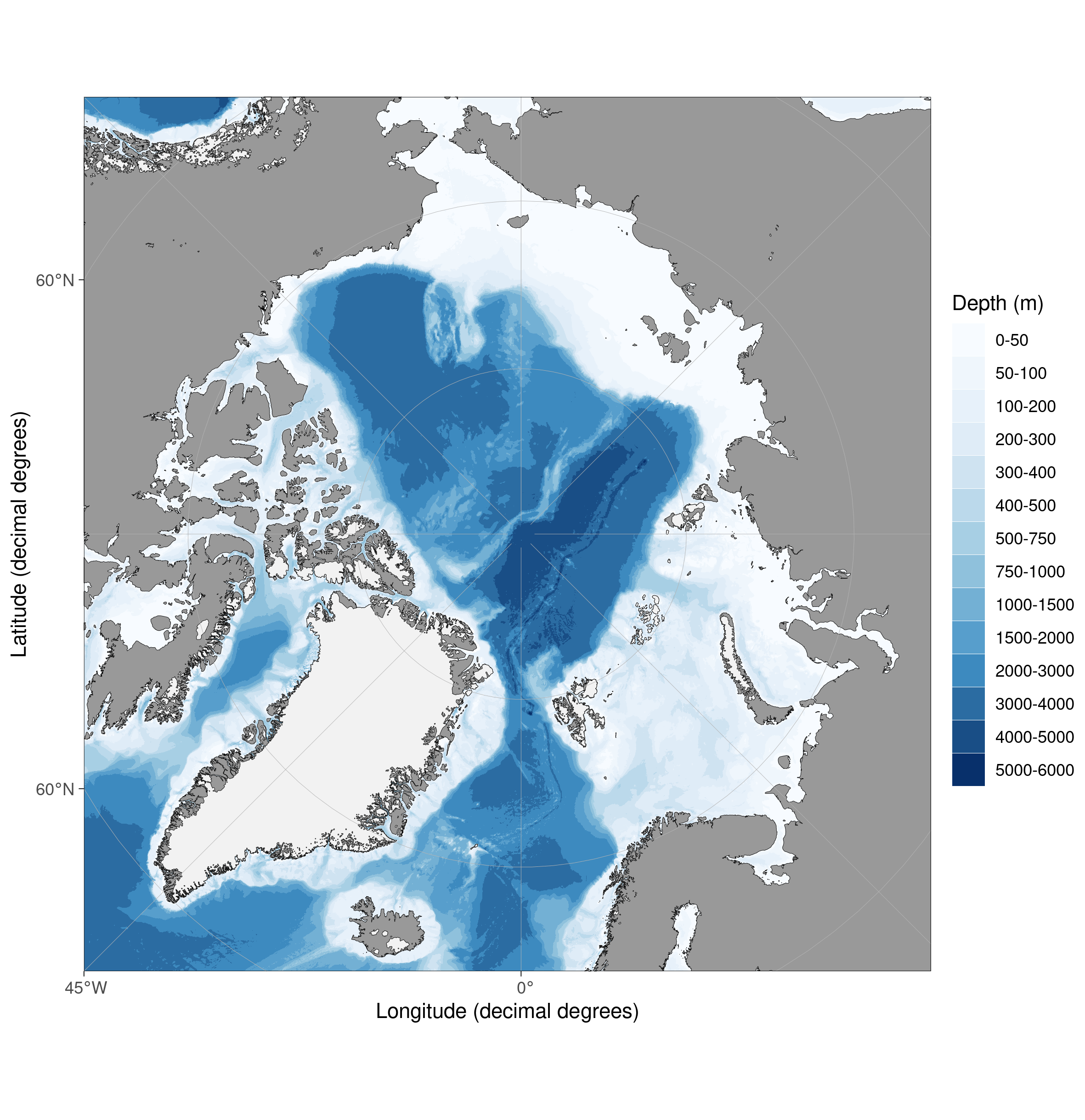
The Arctic (IBCAO)

The IBCAO grid (by GEBCO) vectorized from the North Pole to approximately 60-65°N. A subset of the GEBCO dataset under. Definitely use this one over the GEBCO alternative whenever you can. It is about ten times faster.

basemap("IBCAO", bathymetry = TRUE, glaciers = TRUE)

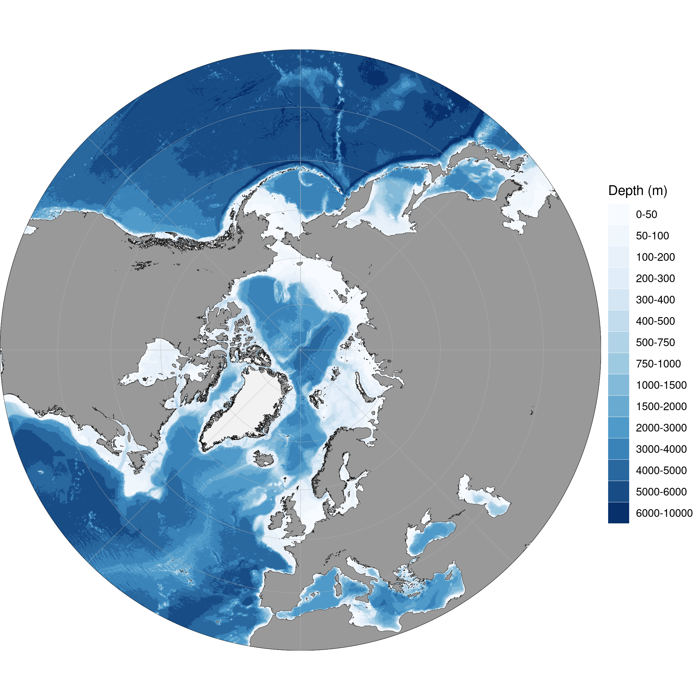
The Northern hemisphere (GEBCO)

The entire GEBCO grid from the North Pole to 10°N vectorized and packed into a >60 Mb R data file. When opened, the data take >3 Gb. This is a clumsy approach and plotting maps using this option can take a long time (up to 10 minutes on a test machine) and will make your computer to beg for mercy. Use this as the last resort and do not blame the package author that you were not warned ;)

basemap("GEBCO", bathymetry = TRUE, glaciers = TRUE)

Geonorge based maps

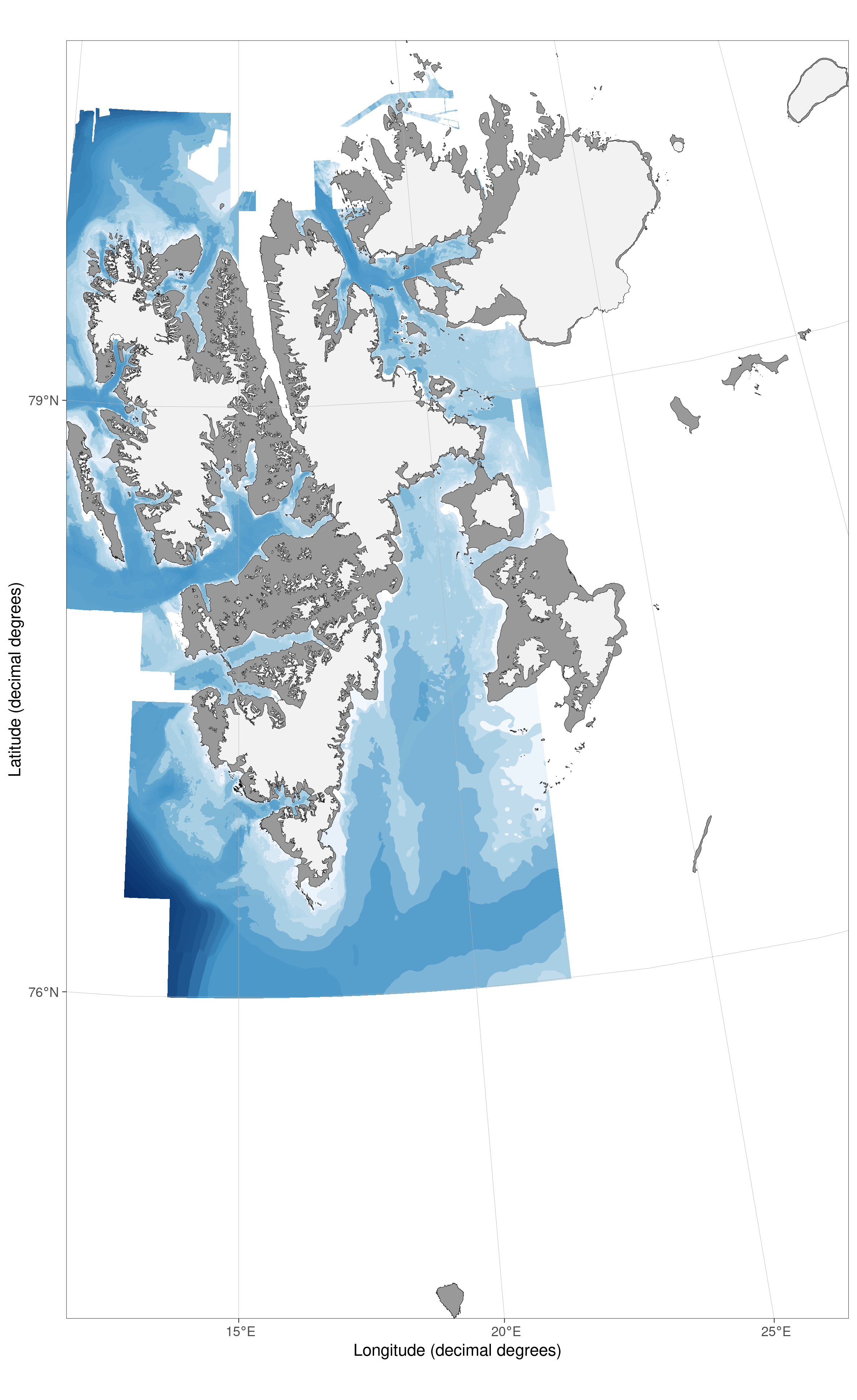
Svalbard

The Svalbard map from the PlotSvalbard package:

basemap("Svalbard", bathymetry = TRUE, glaciers = TRUE)

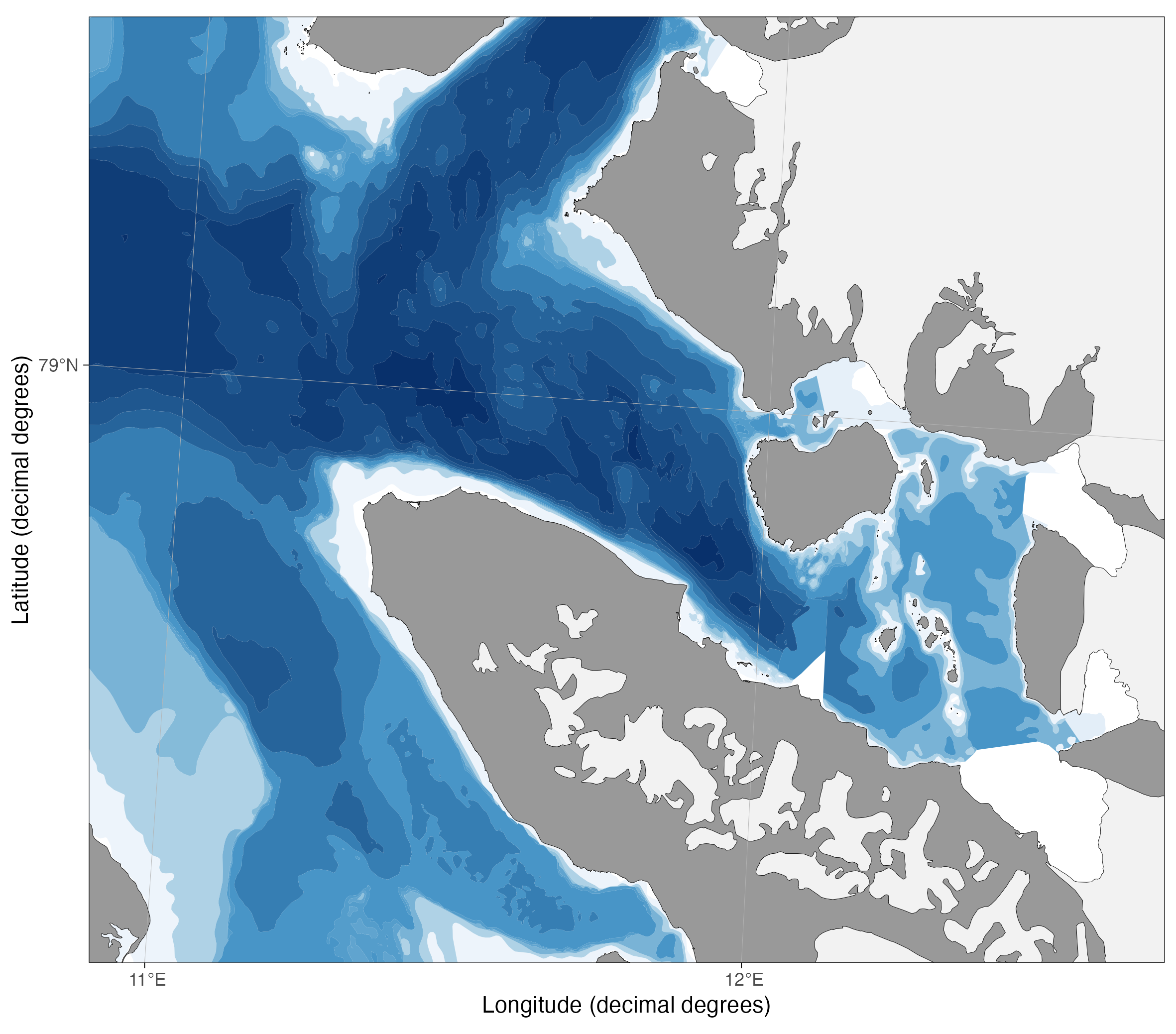
Kongsfjorden from the PlotSvalbard package:

basemap(limits = c(10.9, 12.65, 78.83, 79.12), 
        bathymetry = TRUE, shapefiles = "Svalbard",
        legends = FALSE, glaciers = TRUE)

EMODnet based maps

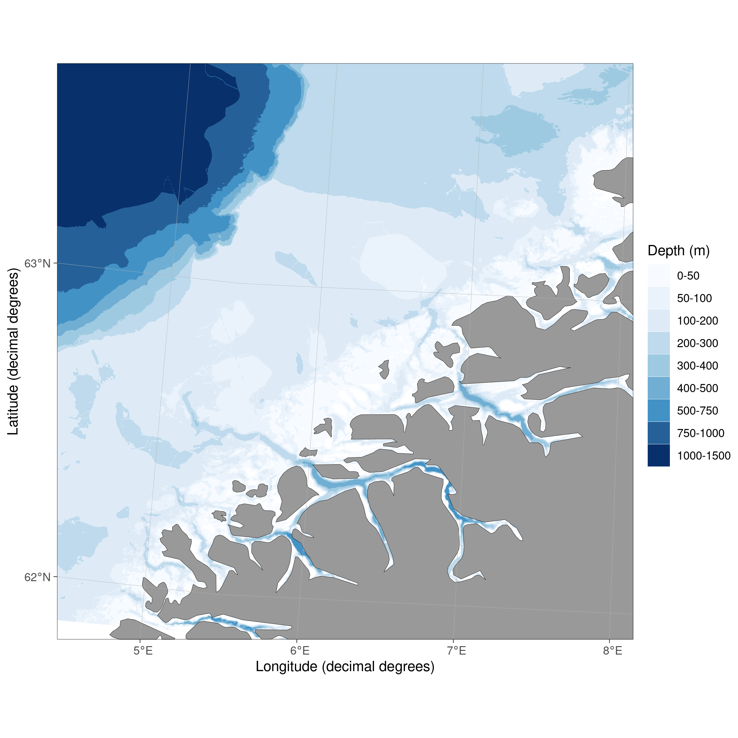
Northeast Atlantic

1/16 arc-minute map over Northeast Atlantic from EMODnet. Might be unfinished. If so and you'll need it, nag the developer.

basemap("EMODnet", bathymetry = TRUE)

MikkoVihtakari/ggOceanMaps documentation built on Oct. 26, 2024, 9:39 a.m.