README.md
In RobinHankin/cmvnorm: The Complex Multivariate Gaussian Distribution
The complex multivariate Gaussian distribution in R

To cite the cmvnorm package in publications please use Hankin (2015).
Consider the (zero mean) multivariate Gaussian distribution with
probability density function
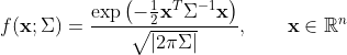
where  is an
is an
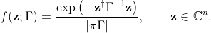
 positive-definite variance matrix. Now compare the complex version with
 Hermitian positive-definite:
See how much nicer the complex version is! No awkward, unsightly factors
of two and no inconvenient square roots. This is essentially due to
Gauss’s integral operating more cleanly over the complex plane than the
real line:

It can be shown that
 ,
so
really is the variance of the distribution. We can also introduce a
nonzero mean,
,
so
really is the variance of the distribution. We can also introduce a
nonzero mean,
 in the natural way. The
 cmvnorm package furnishes some R functionality
for dealing with the complex multivariate Gaussian distribution.
The package in use
The simplest case would be the univariate standard complex normal
distribution, that is is a complex random variable
 with PDF
 .
Random samples are given by
.
Random samples are given by rcnorm():
rcnorm(10)
#>  [1]  0.8930435+0.5399421i -0.2306818-0.5649849i  0.9403101-0.8115161i
#>  [4]  0.8997434-0.2046802i  0.2931958-0.2115770i -1.0889091-0.2909821i
#>  [7] -0.6565960+0.1783489i -0.2083988-0.6306835i -0.0040780+0.3080746i
#> [10]  1.7003467-0.8750718i
Observations are circularly symmetric in the sense that
has the same
distribution as
 for any
 ,
as we may verify visually:
,
as we may verify visually:
par(pty="s")
plot(rcnorm(10000),asp=1,xlim=c(-3,3),ylim=c(-3,3),pch=16,cex=0.2)

We may sample from this distribution and verify that it has zero mean
and unit variance:
z <- rcnorm(1e6)
mean(z)   # zero, subject to sample error
#> [1] -7.22711e-05-1.648871e-04i
var(z)    # one, subject to sample error
#> [1] 1.000039
Note that the real and imaginary components of
have variance
 :
:
z <- rcnorm(1e6)

var(Re(z))
#> [1] 0.4990334
var(Im(z))
#> [1] 0.500692
We may sample from the multivariate case similarly. Suppose
 and
and
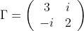 :
:
tm <- c(1,1i)  # true mean
tS <- matrix(c(3,1i,-1i,2),2,2)  # true variance
rcmvnorm(10,mean=tm, sigma=tS)
#>                        [,1]                  [,2]
#>  [1,]  0.7686256-1.0741918i -0.7474151+2.2160427i
#>  [2,]  0.7708602+1.1108247i  0.6358600+1.6525006i
#>  [3,] -1.6582296+0.4285872i  0.5232071+0.2267081i
#>  [4,] -0.8116523+0.7761156i  0.3370565-1.1517968i
#>  [5,]  0.3813992-0.3297815i -0.7391635+1.0239374i
#>  [6,] -1.0306205+0.1980098i -0.2640635+0.0266939i
#>  [7,]  0.0626871-0.1067497i -0.0584202+1.2610072i
#>  [8,] -0.7007527+0.3104665i  0.6747789-0.3943374i
#>  [9,] -0.1592596-1.5369111i  0.9189975-1.1530648i
#> [10,]  1.6842132+0.2346989i  0.9708974+1.5574747i
We may perform elementary inference. For the mean and variance we can
calculate their maximum likelihood estimates:
n <- 1e6  # sample size
z <- rcmvnorm(n,mean=tm, sigma=tS)
colMeans(z)   # should be close to tm=[1,i]
#> [1]  1.000125-0.000710i -0.000733+1.002398i
z <- scale(z,scale=FALSE) # sweep out the mean
cprod(z)/n  # should be close to tS
#>                   [,1]              [,2]
#> [1,] 3.001524+0.00000i 0.001068+1.00205i
#> [2,] 0.001068-1.00205i 2.000310+0.00000i
Further information
For further information, see the package vignette: type
vignette("cmvnorm")
at the R command line.
References
Hankin, R. K. S. 2015. “The complex multivariate Gaussian distribution”.
The R Journal, 7(1):73-80
RobinHankin/cmvnorm documentation built on April 17, 2024, 4:33 p.m.
R Package Documentation
Browse R Packages
We want your feedback!
Note that we can't provide technical support on individual packages. You should contact the package authors for that.
The complex multivariate Gaussian distribution in R
To cite the cmvnorm package in publications please use Hankin (2015).
Consider the (zero mean) multivariate Gaussian distribution with
probability density function
where
is an
positive-definite variance matrix. Now compare the complex version with
Hermitian positive-definite:
See how much nicer the complex version is! No awkward, unsightly factors of two and no inconvenient square roots. This is essentially due to Gauss’s integral operating more cleanly over the complex plane than the real line:
It can be shown that
,
so
really is the variance of the distribution. We can also introduce a
nonzero mean,
in the natural way. The
cmvnorm package furnishes some R functionality
for dealing with the complex multivariate Gaussian distribution.
The package in use
The simplest case would be the univariate standard complex normal
distribution, that is is a complex random variable
with PDF
.
Random samples are given by
rcnorm():
rcnorm(10)
#> [1] 0.8930435+0.5399421i -0.2306818-0.5649849i 0.9403101-0.8115161i
#> [4] 0.8997434-0.2046802i 0.2931958-0.2115770i -1.0889091-0.2909821i
#> [7] -0.6565960+0.1783489i -0.2083988-0.6306835i -0.0040780+0.3080746i
#> [10] 1.7003467-0.8750718i
Observations are circularly symmetric in the sense that
has the same
distribution as
for any
,
as we may verify visually:
par(pty="s")
plot(rcnorm(10000),asp=1,xlim=c(-3,3),ylim=c(-3,3),pch=16,cex=0.2)
We may sample from this distribution and verify that it has zero mean and unit variance:
z <- rcnorm(1e6)
mean(z) # zero, subject to sample error
#> [1] -7.22711e-05-1.648871e-04i
var(z) # one, subject to sample error
#> [1] 1.000039
Note that the real and imaginary components of
have variance
:
z <- rcnorm(1e6)
var(Re(z))
#> [1] 0.4990334
var(Im(z))
#> [1] 0.500692
We may sample from the multivariate case similarly. Suppose
and
:
tm <- c(1,1i) # true mean
tS <- matrix(c(3,1i,-1i,2),2,2) # true variance
rcmvnorm(10,mean=tm, sigma=tS)
#> [,1] [,2]
#> [1,] 0.7686256-1.0741918i -0.7474151+2.2160427i
#> [2,] 0.7708602+1.1108247i 0.6358600+1.6525006i
#> [3,] -1.6582296+0.4285872i 0.5232071+0.2267081i
#> [4,] -0.8116523+0.7761156i 0.3370565-1.1517968i
#> [5,] 0.3813992-0.3297815i -0.7391635+1.0239374i
#> [6,] -1.0306205+0.1980098i -0.2640635+0.0266939i
#> [7,] 0.0626871-0.1067497i -0.0584202+1.2610072i
#> [8,] -0.7007527+0.3104665i 0.6747789-0.3943374i
#> [9,] -0.1592596-1.5369111i 0.9189975-1.1530648i
#> [10,] 1.6842132+0.2346989i 0.9708974+1.5574747i
We may perform elementary inference. For the mean and variance we can calculate their maximum likelihood estimates:
n <- 1e6 # sample size
z <- rcmvnorm(n,mean=tm, sigma=tS)
colMeans(z) # should be close to tm=[1,i]
#> [1] 1.000125-0.000710i -0.000733+1.002398i
z <- scale(z,scale=FALSE) # sweep out the mean
cprod(z)/n # should be close to tS
#> [,1] [,2]
#> [1,] 3.001524+0.00000i 0.001068+1.00205i
#> [2,] 0.001068-1.00205i 2.000310+0.00000i
Further information
For further information, see the package vignette: type
vignette("cmvnorm")
at the R command line.
References
Hankin, R. K. S. 2015. “The complex multivariate Gaussian distribution”. The R Journal, 7(1):73-80
R Package Documentation
Browse R Packages
We want your feedback!
Note that we can't provide technical support on individual packages. You should contact the package authors for that.
Embedding an R snippet on your website
Add the following code to your website.
For more information on customizing the embed code, read Embedding Snippets.