paper.md
In Schuch666/EmissV: Tools for Create Emissions for Air Quality Models
title: 'EmissV: an R package to create vehicular and other emissions for air quality models'
authors:
- affiliation: '1'
name: Daniel Schuch
orcid: 0000-0001-5977-4519
- affiliation: '1'
name: Sergio Ibarra-Espinosa
orcid: 0000-0002-3162-1905
- affiliation: '1'
name: Edmilson Dias de Freitas
orcid: 0000-0001-8783-2747
date: "09 March 2018"
output:
pdf_document: default
bibliography: paper.bib
tags:
- R
- emissions
- air quality model
affiliations:
- index: 1
name: Departamento de Ciências Atmosféricas, Universidade de São Paulo, Brasil
Summary
Air quality models need input data containing information about atmosphere (such as temperature, wind, humidity), terrestrial data (such as terrain, land use, soil types) and emissions. Therefore, the emission inventories are easily seen as the scapegoat if a mismatch is found between modelled and observed concentrations of air pollutants [@PullesHeslinga2010]. The anthropogenic emissions, especially vehicular emissions, are highly dependent on human activity and constantly changing due to various factors ranging from economic (such as the state of conservation of the fleet, renewal of the fleet and the price of fuel) to legal aspects (such as the vehicle routing).
The EmissV is an R package that estimates vehicular emissions by a top-down approach, the emissions are calculated using the statistical description of the fleet at available level (National, State, City, etc). The following steps show an example of the workflow for calculating vehicular emissions, this emissions are initially temporally and spatially disaggregated, and then distributed spatially and temporally to be used as input in numeric air quality models such WRF-Chem [@Grelletal2005].
I. Total: emission of pollutants is estimated from the fleet (number, type and year of vehicles), vehicular activity (km/day) and emission factors (g/km) by pollutant for each interest area (cities, states, countries, etc) or alternatively the totals of some inventory can be used.
II. Spatial distribution: the package has functions to read information from tables, georeferenced images (tiff), shapefiles (sh), openstreetmap data (osm), global inventories in NetCDF format (nc) to calculate point, line and area sources.
III. Emission calculation: calculates the final emission from all different sources and converts to model units and resolution.
IV. Temporal distribution: a set of hourly profiles that represents the mean activity (by hour and day of the week) calculated from traffic counts of toll stations located at São Paulo city available for apply in the emissions.
The package has additional functions for creating emissions from individual sources (including plume rise parameterizations) and to estimate the vehicular emissions of volatile organic compounds from exhaust (through the exhaust pipe), liquid (carter and evaporative) and vapor (fuel transfer operations).
Functions and data
EmissV counts with the folllwing functions:
| Function | Description |
|--------------|-------------------------------------------------------|
| areaSource | Distribution of emissions by area |
| emission | Emissions in the format for atmospheric models |
| emissionFactors | Tool to set-up vehicle emission factors |
| gridInfo | Read grid information from a NetCDF file |
| lineSource | Distribution of emissions by streets |
| perfil | Dataset with temporal profile for vehicular emissions |
| plumeRise | Calculate plume rise height |
| pointSource | Emissions from point sources |
| rasterSource | Distribution of emissions by a georeferenced image |
| read | Read NetCDF data from global inventories |
| streedDist | Distribution by OpenStreetMap street |
| totalEmission| Calculate total emissions |
| totalVOC | Calculate total VOCs emissions |
| vehicles | Tool to set-up vehicle data frame |
Examples
The following example creates an area source for São Paulo State (Brasil). The vehicles function creates a data.frame with information about the São Paulo Fleet using data from [@detran2016], the emissionFactors creates a data.frame with emission factors for CO and PM [@cetesbEV2015]. The totalEmission calculates the total emissions of CO for these vehicles and this emission factors. The next 3 lines opens different data: wrf file, a raster and the area shapefiles. These data are the input for areaSouce that creates an area source based on an image of persistent lights of the Defense Meteorological Satellite Program (DMSP) for São Paulo and Minas Gerais (Brasil) states and finally the function emission calculates the CO emissions.
library(EmissV)

fleet <- vehicles(example = T)
# using a example of vehicles (DETRAN 2016 data and SP vahicle distribution):
#                              Category   Type Fuel      Use       SP ...
# Light Duty Vehicles Gasohol   LDV_E25    LDV  E25  41 km/d 11624342 ...
# Light Duty Vehicles Ethanol  LDV_E100    LDV E100  41 km/d   874627 ...
# Light Duty Vehicles Flex        LDV_F    LDV FLEX  41 km/d  9845022 ...
# Diesel Trucks               TRUCKS_B5 TRUCKS   B5 110 km/d   710634 ...
# Diesel Urban Busses           CBUS_B5    BUS   B5 165 km/d   792630 ...
# Diesel Intercity Busses       MBUS_B5    BUS   B5 165 km/d    21865 ...
# Gasohol Motorcycles          MOTO_E25   MOTO  E25 140 km/d  3227921 ...
# Flex Motorcycles               MOTO_F   MOTO FLEX 140 km/d   235056 ...

# dropping the fleet from Rio de Janeiro (RJ), Parana (PR) and Santa Catarina (SC)
fleet <- fleet[,c(-6,-8,-9)]

EF     <- emissionFactor(example = T)
# using a example emission factor (values calculated from CETESB 2015):
#                                     CO          PM
# Light Duty Vehicles Gasohol  1.75 g/km 0.0013 g/km
# Light Duty Vehicles Ethanol 10.04 g/km 0.0000 g/km
# Light Duty Vehicles Flex     0.39 g/km 0.0010 g/km
# Diesel Trucks                0.45 g/km 0.0612 g/km
# Diesel Urban Busses          0.77 g/km 0.1052 g/km
# Diesel Intercity Busses      1.48 g/km 0.1693 g/km
# Gasohol Motorcycles          1.61 g/km 0.0000 g/km
# Flex Motorcycles             0.75 g/km 0.0000 g/km

TOTAL  <- totalEmission(fleet,EF,pol = c("CO"),verbose = T)
# Total of CO : 1128297.0993334 t year-1

grid   <- gridInfo(paste(system.file("extdata", package = "EmissV"),
                   "/wrfinput_d02",sep=""))
# Grid information from: .../EmissV/extdata/wrfinput_d02

raster <- raster::raster(paste(system.file("extdata", package = "EmissV"),
                         "/dmsp_hi-res.tiff",sep=""))

shape  <- raster::shapefile(paste(system.file("extdata", package = "EmissV"),
                            "/BR.shp",sep=""),verbose = F)[12,1]

Minas_Gerais <- areaSource(shape,raster,grid,name = "Minas Gerais")
# processing Minas Gerais area ...
# fraction of Minas Gerais area inside the domain = 0.0147607845622591

shape  <- raster::shapefile(paste(system.file("extdata", package = "EmissV"),
                            "/BR.shp",sep=""),verbose = F)[22,1]

Sao_Paulo <- areaSource(shape,raster,grid,name = "Sao Paulo")
# processing Sao Paulo area ...
# fraction of Sao Paulo area inside the domain = 0.473260323300595

sp::spplot(raster::merge(drop_units(TOTAL$CO[[1]]) * Sao_Paulo,
                         drop_units(TOTAL$CO[[2]]) * Minas_Gerais),
           scales = list(draw=TRUE),ylab="Lat",xlab="Lon",
           # main=list(label="Emissions of CO [g/d]"),
           col.regions = c("#031638","#001E48","#002756","#003062",
                           "#003A6E","#004579","#005084","#005C8E",
                           "#006897","#0074A1","#0081AA","#008FB3",
                           "#009EBD","#00AFC8","#00C2D6","#00E3F0"))

CO_emissions <- emission(total = TOTAL,
                         pol   = "CO",
                         area  = list(SP = Sao_Paulo, MG = Minas_Gerais),
                         grid  = grid,
                         mm    = 28,
                         plot  = T)
# calculating emissions for CO using molar mass = 28 ...
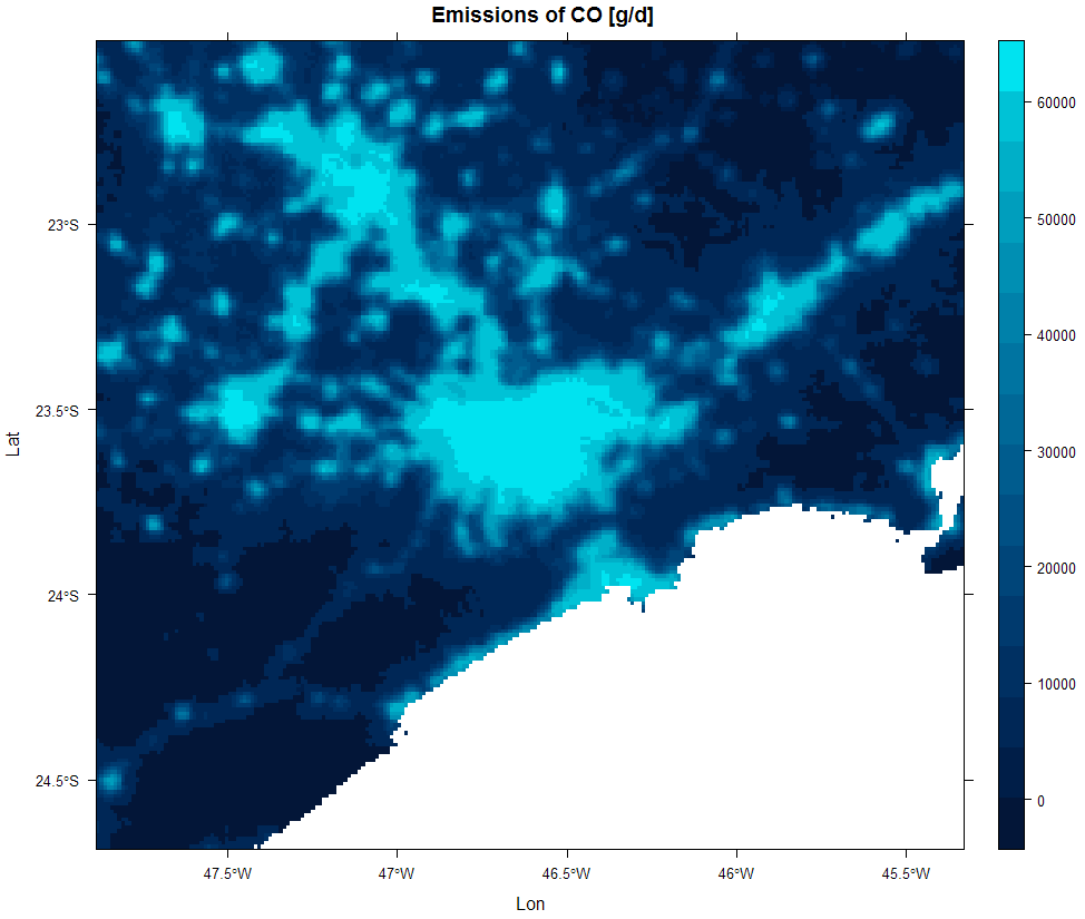
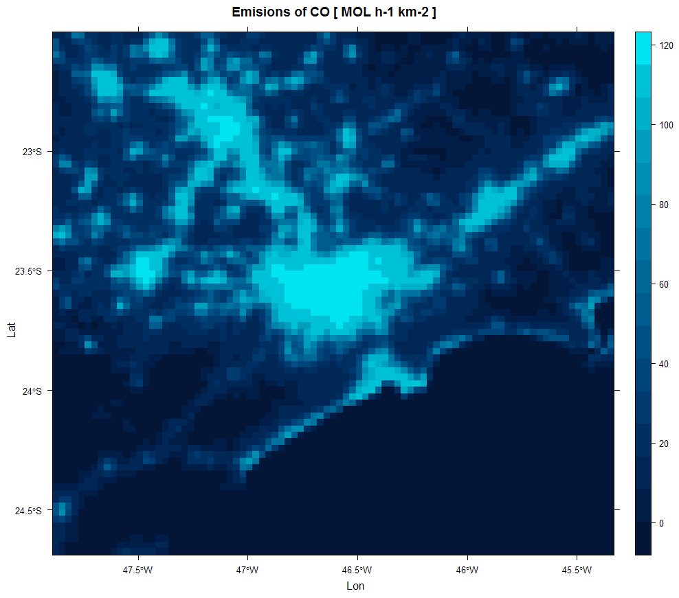
The emissions of CO calculated in this example can be seen in Figure 1 in g/d (by pixel) and the final emissions on Figure 2 in MOL h-1 km-1 (by model grid cell). This emissions can be written to WRF-Chem emission files using some package that makes the interface with NetCDF format such as ncdf4 [@ncdf4], RNetCDF [@RNetCDF], ncdf.tools [@ncdftools] or with the eixport [@eixport]. Some output values (also figures generated by EmissV) might differ slightly depending on the EmissV package-version (as well as different versios of ncdf4, units, raster, sf, lwgeom, etc) and changes to the sample files.
The R package EmissV is available at the repository https://github.com/atmoschem/EmissV.
And this installation is tested automatically on Linux via TravisCI and Windows via Appveyor continuous integration systems. Also, EmissV is already on CRAN https://CRAN.R-project.org/package=EmissV.
Acknowledgements
The development of EmissV was supported by postdoc grans from the Fundação da Universidade de São Paulo and Fundação Coordenação de Aperfeiçoamento de Pessoal de Nível Superior.
References
Schuch666/EmissV documentation built on Sept. 18, 2024, 11:57 p.m.
R Package Documentation
Browse R Packages
We want your feedback!
Note that we can't provide technical support on individual packages. You should contact the package authors for that.
title: 'EmissV: an R package to create vehicular and other emissions for air quality models' authors: - affiliation: '1' name: Daniel Schuch orcid: 0000-0001-5977-4519 - affiliation: '1' name: Sergio Ibarra-Espinosa orcid: 0000-0002-3162-1905 - affiliation: '1' name: Edmilson Dias de Freitas orcid: 0000-0001-8783-2747 date: "09 March 2018" output: pdf_document: default bibliography: paper.bib tags: - R - emissions - air quality model affiliations: - index: 1 name: Departamento de Ciências Atmosféricas, Universidade de São Paulo, Brasil
Summary
Air quality models need input data containing information about atmosphere (such as temperature, wind, humidity), terrestrial data (such as terrain, land use, soil types) and emissions. Therefore, the emission inventories are easily seen as the scapegoat if a mismatch is found between modelled and observed concentrations of air pollutants [@PullesHeslinga2010]. The anthropogenic emissions, especially vehicular emissions, are highly dependent on human activity and constantly changing due to various factors ranging from economic (such as the state of conservation of the fleet, renewal of the fleet and the price of fuel) to legal aspects (such as the vehicle routing).
The EmissV is an R package that estimates vehicular emissions by a top-down approach, the emissions are calculated using the statistical description of the fleet at available level (National, State, City, etc). The following steps show an example of the workflow for calculating vehicular emissions, this emissions are initially temporally and spatially disaggregated, and then distributed spatially and temporally to be used as input in numeric air quality models such WRF-Chem [@Grelletal2005].
I. Total: emission of pollutants is estimated from the fleet (number, type and year of vehicles), vehicular activity (km/day) and emission factors (g/km) by pollutant for each interest area (cities, states, countries, etc) or alternatively the totals of some inventory can be used.
II. Spatial distribution: the package has functions to read information from tables, georeferenced images (tiff), shapefiles (sh), openstreetmap data (osm), global inventories in NetCDF format (nc) to calculate point, line and area sources.
III. Emission calculation: calculates the final emission from all different sources and converts to model units and resolution.
IV. Temporal distribution: a set of hourly profiles that represents the mean activity (by hour and day of the week) calculated from traffic counts of toll stations located at São Paulo city available for apply in the emissions.
The package has additional functions for creating emissions from individual sources (including plume rise parameterizations) and to estimate the vehicular emissions of volatile organic compounds from exhaust (through the exhaust pipe), liquid (carter and evaporative) and vapor (fuel transfer operations).
Functions and data
EmissV counts with the folllwing functions:
| Function | Description | |--------------|-------------------------------------------------------| | areaSource | Distribution of emissions by area | | emission | Emissions in the format for atmospheric models | | emissionFactors | Tool to set-up vehicle emission factors | | gridInfo | Read grid information from a NetCDF file | | lineSource | Distribution of emissions by streets | | perfil | Dataset with temporal profile for vehicular emissions | | plumeRise | Calculate plume rise height | | pointSource | Emissions from point sources | | rasterSource | Distribution of emissions by a georeferenced image | | read | Read NetCDF data from global inventories | | streedDist | Distribution by OpenStreetMap street | | totalEmission| Calculate total emissions | | totalVOC | Calculate total VOCs emissions | | vehicles | Tool to set-up vehicle data frame |
Examples
The following example creates an area source for São Paulo State (Brasil). The vehicles function creates a data.frame with information about the São Paulo Fleet using data from [@detran2016], the emissionFactors creates a data.frame with emission factors for CO and PM [@cetesbEV2015]. The totalEmission calculates the total emissions of CO for these vehicles and this emission factors. The next 3 lines opens different data: wrf file, a raster and the area shapefiles. These data are the input for areaSouce that creates an area source based on an image of persistent lights of the Defense Meteorological Satellite Program (DMSP) for São Paulo and Minas Gerais (Brasil) states and finally the function emission calculates the CO emissions.
library(EmissV)
fleet <- vehicles(example = T)
# using a example of vehicles (DETRAN 2016 data and SP vahicle distribution):
# Category Type Fuel Use SP ...
# Light Duty Vehicles Gasohol LDV_E25 LDV E25 41 km/d 11624342 ...
# Light Duty Vehicles Ethanol LDV_E100 LDV E100 41 km/d 874627 ...
# Light Duty Vehicles Flex LDV_F LDV FLEX 41 km/d 9845022 ...
# Diesel Trucks TRUCKS_B5 TRUCKS B5 110 km/d 710634 ...
# Diesel Urban Busses CBUS_B5 BUS B5 165 km/d 792630 ...
# Diesel Intercity Busses MBUS_B5 BUS B5 165 km/d 21865 ...
# Gasohol Motorcycles MOTO_E25 MOTO E25 140 km/d 3227921 ...
# Flex Motorcycles MOTO_F MOTO FLEX 140 km/d 235056 ...
# dropping the fleet from Rio de Janeiro (RJ), Parana (PR) and Santa Catarina (SC)
fleet <- fleet[,c(-6,-8,-9)]
EF <- emissionFactor(example = T)
# using a example emission factor (values calculated from CETESB 2015):
# CO PM
# Light Duty Vehicles Gasohol 1.75 g/km 0.0013 g/km
# Light Duty Vehicles Ethanol 10.04 g/km 0.0000 g/km
# Light Duty Vehicles Flex 0.39 g/km 0.0010 g/km
# Diesel Trucks 0.45 g/km 0.0612 g/km
# Diesel Urban Busses 0.77 g/km 0.1052 g/km
# Diesel Intercity Busses 1.48 g/km 0.1693 g/km
# Gasohol Motorcycles 1.61 g/km 0.0000 g/km
# Flex Motorcycles 0.75 g/km 0.0000 g/km
TOTAL <- totalEmission(fleet,EF,pol = c("CO"),verbose = T)
# Total of CO : 1128297.0993334 t year-1
grid <- gridInfo(paste(system.file("extdata", package = "EmissV"),
"/wrfinput_d02",sep=""))
# Grid information from: .../EmissV/extdata/wrfinput_d02
raster <- raster::raster(paste(system.file("extdata", package = "EmissV"),
"/dmsp_hi-res.tiff",sep=""))
shape <- raster::shapefile(paste(system.file("extdata", package = "EmissV"),
"/BR.shp",sep=""),verbose = F)[12,1]
Minas_Gerais <- areaSource(shape,raster,grid,name = "Minas Gerais")
# processing Minas Gerais area ...
# fraction of Minas Gerais area inside the domain = 0.0147607845622591
shape <- raster::shapefile(paste(system.file("extdata", package = "EmissV"),
"/BR.shp",sep=""),verbose = F)[22,1]
Sao_Paulo <- areaSource(shape,raster,grid,name = "Sao Paulo")
# processing Sao Paulo area ...
# fraction of Sao Paulo area inside the domain = 0.473260323300595
sp::spplot(raster::merge(drop_units(TOTAL$CO[[1]]) * Sao_Paulo,
drop_units(TOTAL$CO[[2]]) * Minas_Gerais),
scales = list(draw=TRUE),ylab="Lat",xlab="Lon",
# main=list(label="Emissions of CO [g/d]"),
col.regions = c("#031638","#001E48","#002756","#003062",
"#003A6E","#004579","#005084","#005C8E",
"#006897","#0074A1","#0081AA","#008FB3",
"#009EBD","#00AFC8","#00C2D6","#00E3F0"))
CO_emissions <- emission(total = TOTAL,
pol = "CO",
area = list(SP = Sao_Paulo, MG = Minas_Gerais),
grid = grid,
mm = 28,
plot = T)
# calculating emissions for CO using molar mass = 28 ...
The emissions of CO calculated in this example can be seen in Figure 1 in g/d (by pixel) and the final emissions on Figure 2 in MOL h-1 km-1 (by model grid cell). This emissions can be written to WRF-Chem emission files using some package that makes the interface with NetCDF format such as ncdf4 [@ncdf4], RNetCDF [@RNetCDF], ncdf.tools [@ncdftools] or with the eixport [@eixport]. Some output values (also figures generated by EmissV) might differ slightly depending on the EmissV package-version (as well as different versios of ncdf4, units, raster, sf, lwgeom, etc) and changes to the sample files.
The R package EmissV is available at the repository https://github.com/atmoschem/EmissV. And this installation is tested automatically on Linux via TravisCI and Windows via Appveyor continuous integration systems. Also, EmissV is already on CRAN https://CRAN.R-project.org/package=EmissV.
Acknowledgements
The development of EmissV was supported by postdoc grans from the Fundação da Universidade de São Paulo and Fundação Coordenação de Aperfeiçoamento de Pessoal de Nível Superior.
References
R Package Documentation
Browse R Packages
We want your feedback!
Note that we can't provide technical support on individual packages. You should contact the package authors for that.
Embedding an R snippet on your website
Add the following code to your website.
For more information on customizing the embed code, read Embedding Snippets.