README.md

In YTLogos/ttplot: Tao Yan's Plot Toolkit

Overview

This package is just developed to finish my project. So most of scripts are NOT stable enough. By wrapping some functions from other useful packages, it's easy for us to finish our jobs.

Installation

This package dependents on some other packages:vcfR,dplyr,genetics,LDheatmap, ...

The dependent packages will be installed at the time you install the package ttplot

#install the ttplot package from Github
if(!require(devtools)) {
  install.packages("devtools"); 
  require(devtools)
} 
devtools::install_github("YTLogos/ttplot")

Usage

Until now there are just several functions

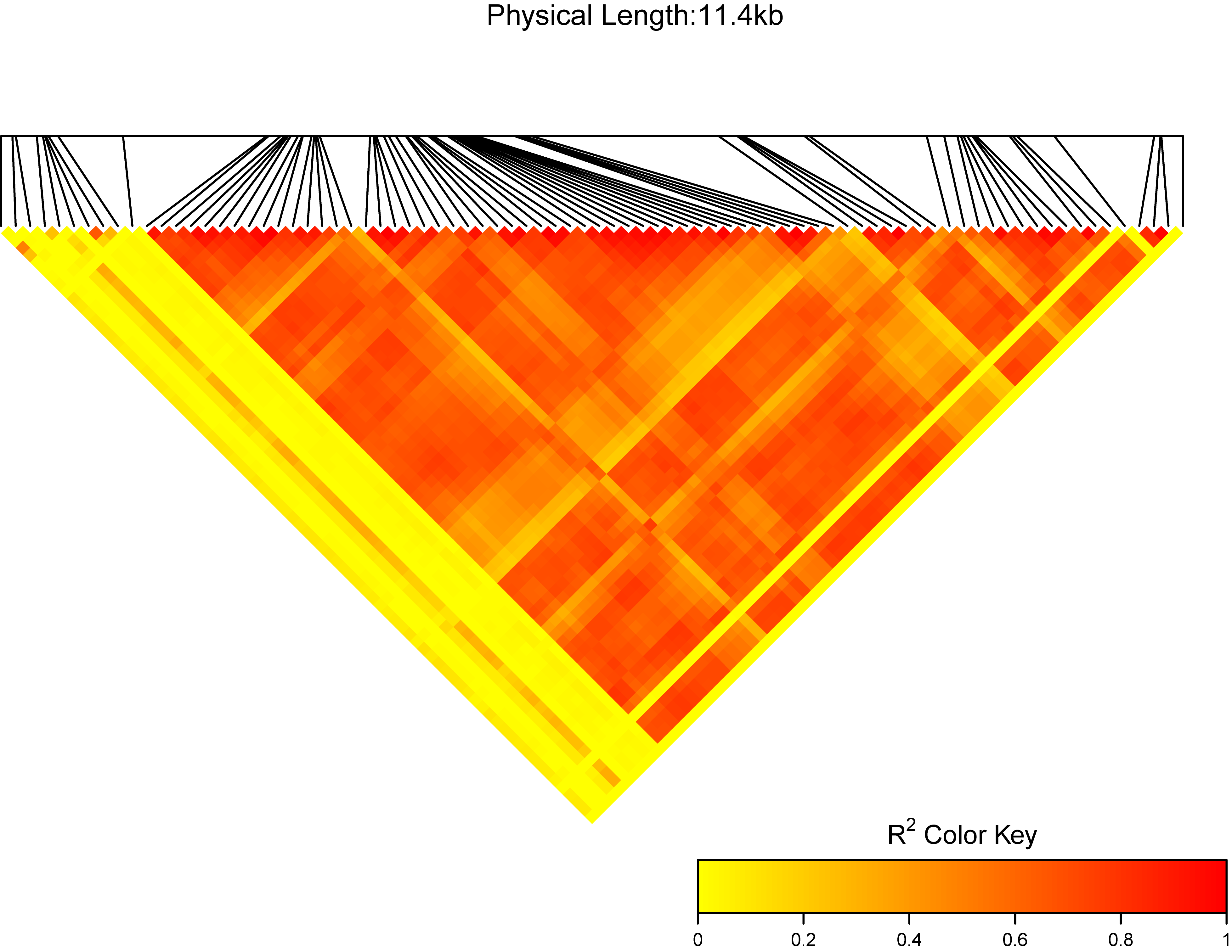
Draw the LDheatmap from the VCF format file (plink format)

VCF (Variant Call Format) is a text file format. It contains meta-information lines, a header line, and then data lines each containing information about a position in the genome. There is an example how to draw LDheatmap from data in VCF file(plink format). The VCF file looks like:

#This is a test vcf file (test.vcf) 

##fileformat=VCFv4.3
##fileDate=20090805
##source=myImputationProgramV3.1
##reference=file:///seq/references/1000GenomesPilot-NCBI36.fasta
##contig=<ID=20,length=62435964,assembly=B36,md5=f126cdf8a6e0c7f379d618ff66beb2da,species="Homo sapiens",taxonomy=x>
##phasing=partial
##INFO=<ID=NS,Number=1,Type=Integer,Description="Number of Samples With Data">
##INFO=<ID=DP,Number=1,Type=Integer,Description="Total Depth">
##INFO=<ID=AF,Number=A,Type=Float,Description="Allele Frequency">
##INFO=<ID=AA,Number=1,Type=String,Description="Ancestral Allele">
##INFO=<ID=DB,Number=0,Type=Flag,Description="dbSNP membership, build 129">
##INFO=<ID=H2,Number=0,Type=Flag,Description="HapMap2 membership">
##FILTER=<ID=q10,Description="Quality below 10">
##FILTER=<ID=s50,Description="Less than 50% of samples have data">
##FORMAT=<ID=GT,Number=1,Type=String,Description="Genotype">
##FORMAT=<ID=GQ,Number=1,Type=Integer,Description="Genotype Quality">
##FORMAT=<ID=DP,Number=1,Type=Integer,Description="Read Depth">
##FORMAT=<ID=HQ,Number=2,Type=Integer,Description="Haplotype Quality">
#CHROM POS      ID         REF   ALT    QUAL  FILTER   INFO                             FORMAT       NA00001         NA00002          NA00003
20     14370    rs6054257  G     A      29    PASS    NS=3;DP=14;AF=0.5;DB;H2           GT:GQ:DP:HQ  0|0:48:1:51,51  1|0:48:8:51,51   1/1:43:5:.,.
20     17330    .          T     A      3     q10     NS=3;DP=11;AF=0.017               GT:GQ:DP:HQ  0|0:49:3:58,50  0|1:3:5:65,3     0/0:41:3
20     1110696  rs6040355  A     G,T    67    PASS    NS=2;DP=10;AF=0.333,0.667;AA=T;DB GT:GQ:DP:HQ  1|2:21:6:23,27  2|1:2:0:18,2     2/2:35:4
20     1230237  .          T     .      47    PASS    NS=3;DP=13;AA=T                   GT:GQ:DP:HQ  0|0:54:7:56,60  0|0:48:4:51,51   0/0:61:2
20     1234567  microsat1  GTC   G,GTCT 50    PASS    NS=3;DP=9;AA=G                    GT:GQ:DP     0/1:35:4        0/2:17:2         1/1:40:3

This kind of VCF is very large, so first we can use plink to recode the VCF file

$ plink --vcf test.vcf --recode vcf-iid --out Test -allow-extra-chr

So the final VCF file we will use looks like：

##fileformat=VCFv4.2
##fileDate=20180905
##source=PLINKv1.90
##contig=<ID=chrC07,length=31087537>
##INFO=<ID=PR,Number=0,Type=Flag,Description="Provisional reference allele, may not be based on real reference genome">
##FORMAT=<ID=GT,Number=1,Type=String,Description="Genotype">
#CHROM  POS ID  REF ALT QUAL    FILTER  INFO    FORMAT  R4157   R4158
chrC07  31076164    .   T   G   .   .   PR  GT  0/0 0/1
chrC07  31076273    .   G   A   .   .   PR  GT  0/0 0/1
chrC07  31076306    .   G   T   .   .   PR  GT  0/0 0/0

In the extdata directory there is one test file: test.vcf. We can test the function:

library(ttplot)
test <- system.file("extdata", "test.vcf", package = "ttplot")
ttplot::MyLDheatMap(vcffile = test, title = "My gene region")

More

Usage:

MyLDheatMap(vcffile, file.output = TRUE, file = "png",
  output = "region", title = "region:", verbose = TRUE, dpi = 300)

Arguments

• vcffile: The plink format vcf file. More detail can see View(test_vcf).
• file.output: a logical, if file.output=TRUE, the result will be saved. if file.output=FALSE, the result will be printed. The default is TRUE.
• file: a character, users can choose the different output formats of plot, so far, "jpeg", "pdf", "png", "tiff" can be selected by users. The default is "png".
• title: a character, the title of the LDheatmap will be "The LDheatmap of title". the default is "region:". I suggest users use your own title.
• verbose: whether to print the reminder.
• dpi: a number, the picture element for .jpeg, .png and .tiff files. The default is 300.

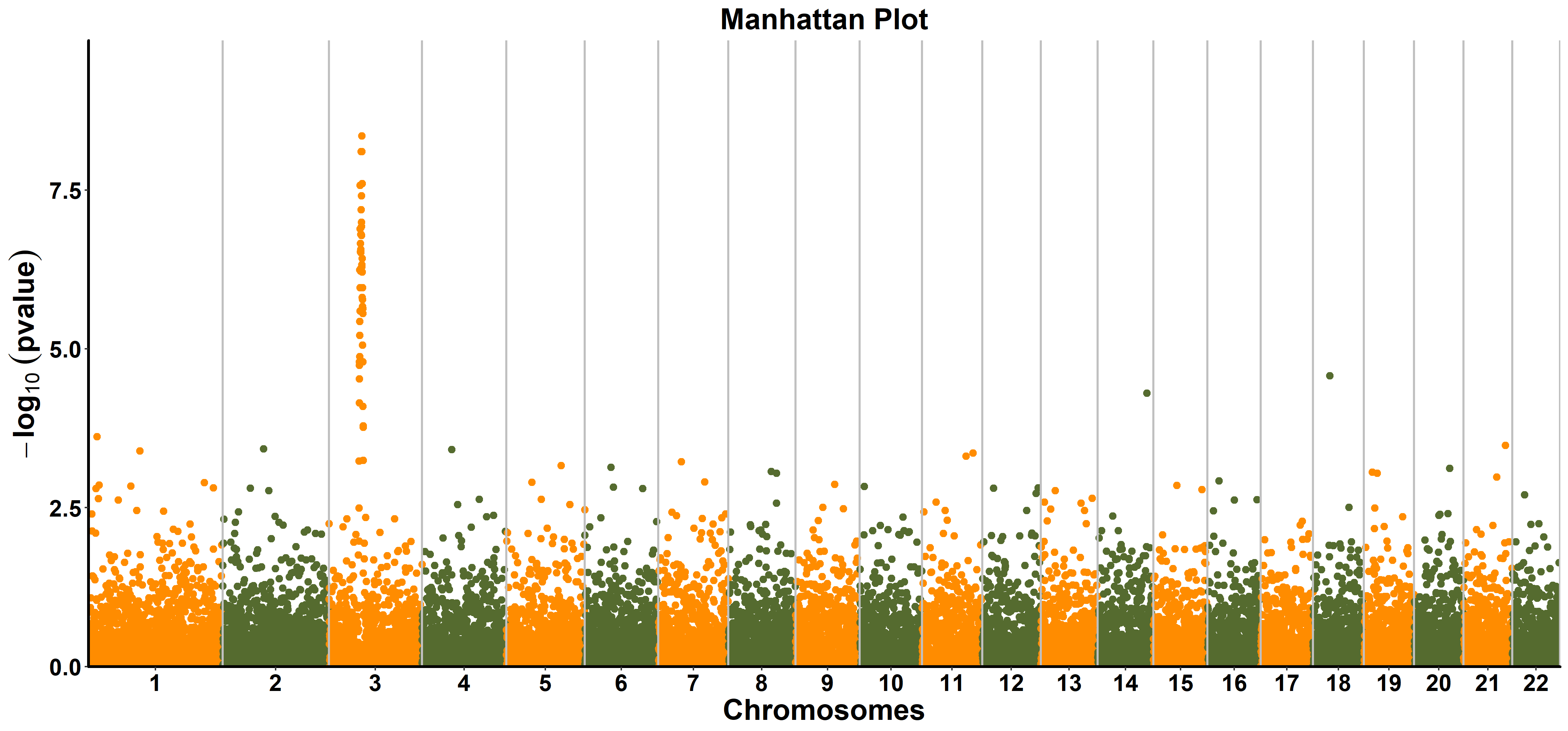
ggmanhattan(): make manhattan plot based on ggplot2

Here, we will use the data gwasResults from R package qqman. This function is provided to make manhattan plot with full ggplot customizability. So next we can customize the manhattan plot with kinds of functions of ggplot2 and add additional layers. The data need be reshaped as following:

> head(gwasResults)
  SNP CHR BP         P
1 rs1   1  1 0.9148060
2 rs2   1  2 0.9370754
3 rs3   1  3 0.2861395
4 rs4   1  4 0.8304476
5 rs5   1  5 0.6417455
6 rs6   1  6 0.5190959

Then use the function ggmanhattan from ttplot to make a manhattan plot:

ttplot::ggmanhattan(gwasResults)

More

ggmanhattan(gwasres, snp = NA, bp = NA, chrom = NA, pvalue = NA,
  index = NA, file.output = FALSE, file = "png", output = "Trait",
  dpi = 300, vlinetype = "solid", vlinesize = 0.75,
  title = "Manhattan Plot", color = c("#FF8C00", "#556B2F"),
  pointsize = 1.25, verbose = TRUE, ...)

Arguments

• gwasres a data frame of gwas results.
• snp Name of the column containing SNP identifiers; default is 'snp'.
• bp Name of the column containing the SNP positions; default is 'bp'.
• chrom Name of the column containing the chromosome identifers; default is 'chrom'.
• pvalue Name of the column containing the p values; default is 'pvalue'.
• file.output a logical, if file.output=TRUE, the result will be saved. if file.output=FALSE, the result will be printed. The default is TRUE.
• file a character, users can choose the different output formats of plot, so far, "jpeg", "pdf", "png", "tiff" can be selected by users. The default is "png".
• dpi a number, the picture element for .jpeg, .png and .tiff files. The default is 300.
• vlinetype the type of vline (geom_vline()). The default is "solid".
• vlinesize the size of the vline. The default is 0.75.
• title the title of manhattan plot. The default is "Manhattan Plot".
• color the colors of alternate chromosome. The default is c("#FF8C00", "#556B2F").
• pointsize the size of point. The default is 1.25.

Get genes bsaed on the locations of significant SNPs

This function need two input files: gff, snp.

library(ttplot)
gff <- read.table(system.file("extdata", "test.gff", package = "ttplot"), header= TRUE)
head(gff)

chr  start    end          gene
1 436789 437474 chrA01g000077
1 439907 442623 chrA01g000078
1 448692 449999 chrA01g000079
1 454920 456931 chrA01g000080
1 457568 460619 chrA01g000081
1 461129 462693 chrA01g000082

snp <- read.table(system.file("extdata", "test_sig_snp.txt", package = "ttplot"), header= TRUE)
head(snp)

SNP CHR       BP        P
1_500000   1   500000 5.53e-11
1_650000   1   650000 7.04e-09
2_1880000   2  1880000 3.84e-09
3_30500000   3 30500000 7.57e-08

Then we can get the candidate genes in regions based on significant SNPs of GWAS results.

ttplot::get_gene_from_snp(gff = gff, sig.snp = snp, distance = 20000, file.save = FALSE)
The distance you choose is 20000bp!
You have 4 significant SNPs and 130 genes!
Now we will extract the genes in the significant regions! This will need some time, please wait for severals minutes! ...

The result is : 
-------------------------------------------------------------
# A tibble: 9 x 5
chrom geneid        gene_start gene_end snp_location
<dbl> <chr>              <dbl>    <dbl>        <dbl>
1 chrA01g000088     479923   485997       500000
1 chrA01g000089     495531   497917       500000
1 chrA01g000090     498488   499689       500000
1 chrA01g000091     499749   501301       500000
1 chrA01g000092     503622   507079       500000
1 chrA01g000093     507659   510321       500000
1 chrA01g000094     515103   516863       500000
1 chrA01g000095     517335   518776       500000
1 chrA01g000096     519020   520668       500000

More

Usage
get_gene_from_snp(gff, sig.snp, distance = 50000, file.save = TRUE,
  file.type = "csv", gff.chrom = NA, snp.chrom = NA, geneid = NA,
  pvalue = NA, gene_start = NA, gene_end = NA, snp_location = NA,
  verbose = TRUE, ...)

Arguments

• gff: a data frame of all the gene (transcript), must have column names.
• sig.snp: a data frame of significant SNPs.
• distance: numeric (bp), it is to define the region. The default is 50000, you need to choose it based on the LD distance in your study.
• file.save: a logical, if file.output=TRUE, the result will be saved. if file.output=FALSE, the result will be printed. The default is TRUE.
• file.type: a character, users can choose the different output formats, so far, "csv", "txt", "xlsx" can be selected by users. The default is "csv".
• gff.chrom: Name of the column containing the chromosome identifers in the gff file; default is NA.
• snp.chrom: Name of the column containing the chromosome identifers in the snp.sig file; default is NA.
• geneid: Name of the column containing the geneid in gff file; default is NA.
• pvalue: Name of the column containing the p values in snp.sig file; default is NA.
• snp_location: Name of the column containing the snp position in snp.sig file; default is NA.

YTLogos/ttplot documentation built on Aug. 20, 2019, 8:18 p.m.