README.md

In brshallo/piececor: Tidy Piecewise Correlations

piececor

• Steps
• Example
  • Correlations of segments
  • Plots of splits
  • Weighted correlation
• Customizing
  • Smoother fit
  • Correlation metric
• Installation
• Limitations & Notes
• Resources

piececor is a toy package for calculating piecewise correlations of a set of {variables of interest} with a {target} variable. This may be useful for exploratory data analysis or in “simple filtering” of features for predictive modeling.

This package is a rough mock-up of initial ideas discussed between Bryan Shalloway, Dr. Shaina Race, and Ricky Tharrington.

Steps

The core function is piecewise_cors() which, for each {variable of interest}:

1. Splits observations into segments based on the local minima / maxima of a smoother fit on {target} \~ {variable of interest}.
2. Calculates the correlation between {target} & {variable of interest} for each segment
3. Allows for calculating a weighted correlation coefficient across segments
4. Repeat for all {variables of interest} with {target}

Example

Use a version of mtcars data with some numeric columns converted to factors.

library(tidyverse)
library(piececor)

min_unique_to_fact <- function(x, min_unique = 8){
  if( (length(unique(x)) < min_unique) & is.numeric(x) ){
    return(as.factor(x))
  } else x
}

mtcars_neat <- mtcars %>%
  as_tibble(rownames = "car") %>%
  mutate(across(where(is.numeric), min_unique_to_fact))

Correlations of segments

Specify data, .target, and ...[1]

mods_cors <- piecewise_cors(data = mtcars_neat,
                            .target = hp,
                            mpg, disp, drat, wt, qsec)

Note that tidy selectors can be used in place of explicitly typing each variable of interest. I.e. in the above example mpg, disp, drat, wt, qseccould be replaced by where(is.double).

piecewise_cors() returns a named list of mods and cors.

Correlations:

For each variable of interest, cors has a dataframe with information on the domain (gtoe to lt) for each segment of observations (data), the number of observations (n_obs) in the segment, and the associated correlation (cor) of the variable with .target.

(cors dataframes with one row represent smoothed fits with no local minima / maxima.)

mods_cors$cors
#> $mpg
#> # A tibble: 1 x 5
#>    gtoe    lt data              n_obs    cor
#>   <dbl> <dbl> <list>            <dbl>  <dbl>
#> 1  -Inf   Inf <tibble [32 x 2]>    32 -0.895
#> 
#> $disp
#> # A tibble: 1 x 5
#>    gtoe    lt data              n_obs   cor
#>   <dbl> <dbl> <list>            <dbl> <dbl>
#> 1  -Inf   Inf <tibble [32 x 2]>    32 0.851
#> 
#> $drat
#> # A tibble: 1 x 5
#>    gtoe    lt data              n_obs    cor
#>   <dbl> <dbl> <list>            <dbl>  <dbl>
#> 1  -Inf   Inf <tibble [32 x 2]>    32 -0.520
#> 
#> $wt
#> # A tibble: 1 x 5
#>    gtoe    lt data              n_obs   cor
#>   <dbl> <dbl> <list>            <dbl> <dbl>
#> 1  -Inf   Inf <tibble [32 x 2]>    32 0.775
#> 
#> $qsec
#> # A tibble: 4 x 5
#>     gtoe    lt data              n_obs    cor
#>    <dbl> <dbl> <list>            <int>  <dbl>
#> 1 -Inf    16.7 <tibble [6 x 2]>      6 -0.841
#> 2   16.7  17.6 <tibble [10 x 2]>    10  0.837
#> 3   17.6  19.4 <tibble [9 x 2]>      9 -0.727
#> 4   19.4 Inf   <tibble [7 x 2]>      7  0

By default piecewise_cors() uses Spearman’s Rank Correlation Coefficient[2].

Smoothing models:

For each variable of interest, mods contains a parsnip fit object (the smoothing model). The local minima / maxima of these fitted models determines the breakpoints for segmenting observations for each correlation calculation[3]. In our example, these may be accessed with mods_cors$mods.

By default mgcv::gam() (via a parsnip interface) is the engine for the smoother. At present, it is also the only model type that will work[4].

Plots of splits

To review the split points, the outputs from piecewise_cors() can be passed into plot_splits(). Variables of interest that you wish to plot must be typed or specified by a tidy selector.

mods_cors %>% 
  plot_splits(mpg, qsec)
#> mpg: No splits, i.e. no local extrema in smoothed fit.
#> $mpg

#> 
#> $qsec

To view plots for all variables of interest, replace mpg, qsec with everything().

Weighted correlation

The output from piecewise_cors() can be passed to the helper weighted_abs_mean_cors() to calculate an overall weighted “correlation” between 0 and 1 for each variable of interest.

weighted_cors <- weighted_abs_mean_cors(mods_cors)

weighted_cors
#> # A tibble: 5 x 2
#>   name  value
#>   <chr> <dbl>
#> 1 mpg   0.895
#> 2 disp  0.851
#> 3 drat  0.520
#> 4 wt    0.775
#> 5 qsec  0.700

weighted_cors %>% 
  mutate(name = forcats::fct_reorder(name, value)) %>% 
  ggplot(aes(y = name, x = value))+
  geom_col()+
  xlim(c(0, 1))+
  labs(title = "Weighted correlation with 'hp'")

By default a Fisher transformation is applied to the individual correlations when calculating the weighted correlation. See ?weighted_abs_mean_cors for more information.

See the end of section Correlation metric for an example calculating a p-value on piecewise correlations.

Customizing

Arguments custom_model_spec and fit_formula can be used to customize the Smoother fit. cor_function allows for changes in the Correlation metric calculated on the segments. See ?piecewise_cors for more detail on these arguments.

Smoother fit

custom_model_spec can take in a parsnip model specifications[5]. For example, setting sp (smoothing parameter) to sp = 2 gives a smoother fit to hp ~ qsec that no longer segments the observations:

mod_spec <- parsnip::gen_additive_mod() %>%
  parsnip::set_engine("mgcv", method = "REML", sp = 2) %>%
  parsnip::set_mode("regression")

mods_cors_custom <- 
  piecewise_cors(data = mtcars_neat,
                 .target = hp,
                 mpg, disp, drat, wt, qsec,
                 custom_model_spec = mod_spec)

mods_cors_custom %>% 
  plot_splits(qsec)
#> qsec: No splits, i.e. no local extrema in smoothed fit.
#> $qsec

Equivalently, this may be specified by passing the parameter into the fit_formula argument:

# Chunk not evaluated
piecewise_cors(
  data = mtcars_neat,
  .target = hp,
  mpg, disp, drat, wt, qsec,
  fit_formula = ".target ~ s(..., sp = 2)"
)

See Generalized additive models via mgcv and associated reference pages for more details on parsnip interfaces.

Correlation metric

Say you want to measure Pearson’s rather than Spearman’s correlation coefficient on segments, you could use the cor_function argument to change the lambda function:

piecewise_cors(
  data = mtcars_neat,
  .target = hp,
  mpg, disp, drat, wt, qsec,
  cor_function = "~cor(.x, method = 'pearson')[2,1]"
) %>%
  weighted_abs_mean_cors()
#> # A tibble: 5 x 2
#>   name  value
#>   <chr> <dbl>
#> 1 mpg   0.776
#> 2 disp  0.791
#> 3 drat  0.449
#> 4 wt    0.659
#> 5 qsec  0.718

You aren’t prevented from passing into cor_function lambda functions[6] to calculate metrics/statistics other than correlations[7].

For example, say we want to see the p.value’s of Pearson correlations[8] at each segment for hp ~ qsec:

# Warnings silenced in chunk output
mods_cors_pvalues <- 
  piecewise_cors(data = mtcars_neat,
                 .target = hp,
                 mpg, disp, drat, wt, qsec,
# cor.test() expects x and y vectors not a matrix or dataframe
                 cor_function = "~cor.test(.x[[1]], .x[[2]], method = 'pearson')$p.value"
  )

# let's check for qsec
mods_cors_pvalues$cors$qsec
#> # A tibble: 4 x 5
#>     gtoe    lt data              n_obs     cor
#>    <dbl> <dbl> <list>            <int>   <dbl>
#> 1 -Inf    16.7 <tibble [6 x 2]>      6 0.0394 
#> 2   16.7  17.6 <tibble [10 x 2]>    10 0.0156 
#> 3   17.6  19.4 <tibble [9 x 2]>      9 0.00489
#> 4   19.4 Inf   <tibble [7 x 2]>      7 0.660

The cor column here actually represents the statistical test (run separately on each segment) of the null hypothesis that the correlation coefficient is 0.

We could use Stouffer’s Z-score method to combine these into an overall p-value:

# combine_test() is (mostly) copied from {survcomp} package
mods_cors_pvalues$cors$qsec %>% 
  with(piececor:::combine_test(cor, n_obs, method = "z.transform"))
#> [1] 0.0006511026

Installation

Install from github with:

devtools::install_github("brshallo/piececor")

Limitations & Notes

• Very slow compared to other common “simple filtering” methods for predictive modeling[9].
• Trying on a few different datasets, it often does not pass the “eye test”.
  • Splits often come near flatter parts of the data or at the tails of the distribution where there are fewer points
• {piececor} is intended for when trying to measure non-linear and non-monotonic associations. If the relationships are likely monotonic, generally using either Spearman’s or Kendall’s correlation coefficients is a better + faster option[10].
• Changing default correlation method from Spearman’s to Kendall’s probably makes sense (as Kendall’s has better statistical properties – particularly regarding calculating p-values), though I should verify that Fisher’s transformation can also be used with Kendall’s method[11].
• Output of weighted_abs_mean_cors() is not particularly meaningful in a traditional notion of “correlation.”
  • Splits are determined based on optimizing a fit to a {target} – therefore flipping {target} \~ {variable of interest} to {variable of interest} \~ {target} produces different weighted correlation scores[12]. A smoother that was fit based on total least squares or minimizing orthogonal distance or some other approach may be more appropriate.
• How to do weighted correlation metrics and associated p-values generally should be given a bit more thought.
  • Other resources on “simple filtering” techniques (e.g. from Feature Engineering and Selection…) recommend converting scores of feature importance to some standardized metric, e.g. a p-value.
• There is extensive literature in predictive modeling on identifying knots. The experiment with this package is to take advantage of existing software that uses knots or other smoothing techniques and then instead to consider the local minima / maxima created by those techniques to inform cut-points. The defaults of “mgcv” hopes to prevent overfitting and the use of “Spearman’s” correlation means we’re checking whether the relationship is monotonic.
  • However we haven’t done a ton of research on relevant literature concerning knots and other methods for determining cut-points.
  • Right now the cut-points are essentially determined by looking where in the smoothed fits the first derivative == 0. We may want to consider critical points or other methods. We may also want to have some level of tolerance or requisite change in slope or observations in segment, etc. so that minor bumps don’t create multiple segments.
• custom_model_spec allows a parsnip model specification, with the idea that this would facilitate the input of any kind of smoother supported by parsnip (e.g. MARS, polynomial regression, …). However actually implementing this would require the removal of the dependency on gratia as well as multiple other changes to piececor.
• More thought should go into the structure of the output of piecewise_cors()
• (Almost) no checks, tests, catches, etc. have been set-up

Resources

Links are copied from slack discussions[13] and may be only tangentially related to piececor package.

• Within the easystats ecosystem is the correlation package / function that supports Distance correlation that measures both linear and non-linear associations.
• The infotheo package supports measuring the amount of mutual information between variables.
• NNS Package for Nonlinear nonparametric statistics, related to kernel regression techniques (python package also available).
• ppsr R implementation of predictive power score which outputs a normalized score of how well x predicts y (using a particular model specification and choice of performance metric) – python package is also available.
• ProcessMiner/nlcor package (non-linear correlation)[14].

I ran a rough speed test on these methods here:

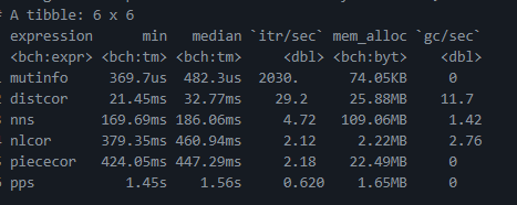
• See gist for speed tests on above packages and piececor.
• For tidy interface for measures of association also see infer, corrr, easystats
• Just slightly tangential, there are a ton of non-linear projection methods out there, e.g. KPCA, UMAP, ICA, tSNE, and many others… many of these are accessible via recipes or embed packages in tidymodels ecosystem.
• “Variable Importance Analysis: A Comprehensive review” https://www.sciencedirect.com/science/article/abs/pii/S0951832015001672
• “Permutation importance: a corrected feature importance measure” https://academic.oup.com/bioinformatics/article/26/10/1340/193348?login=true
• “A computationally fast variable importance test for random forests for high-dimensional data” https://core.ac.uk/download/pdf/216462194.pdf
• ELI5 python package: https://eli5.readthedocs.io/en/latest/overview.html#basic-usage
• “How To Assess Statistical Significance In Your Data with Permutation Tests” https://towardsdatascience.com/how-to-assess-statistical-significance-in-your-data-with-permutation-tests-8bb925b2113d
• “Interpretable Machine Learning” https://christophm.github.io/interpretable-ml-book/
• Getting derivitives from GAM’s
  • https://gavinsimpson.github.io/gratia/reference/fderiv.html
  • https://stackoverflow.com/questions/14207250/determining-derivatives-from-gam-smooth-object
• Covariant Derivatives https://en.wikipedia.org/wiki/Covariant_derivative
• “Efficient test for nonlinear dependence of two continuous variables” https://bmcbioinformatics.biomedcentral.com/articles/10.1186/s12859-015-0697-7
• 11.2 Simple Filters, from Feature Engineering and Selection… http://www.feat.engineering/greedy-simple-filters.html
• Fisher transformation https://en.wikipedia.org/wiki/Fisher_transformation
• Parsnip package documentation on generalized additive models: https://parsnip.tidymodels.org/reference/details_gen_additive_mod_mgcv.html

[1] variables of interest are represented by ... in the function.

[2] So is measuring the extent to which the relationship is monotonic.

[3] mods is primarily saved simply for use with piececor::plot_splits().

[4] In theory, with some changes, other model types with parsnip interfaces could be added with minimal effort

[5] Again only generative additive models via the “mgcv” engine may be specified. This is in large part due to a dependency on the deprecated fderiv() function in gratia. Though changes would also need to be made to the fit_formula argument in piececor::piecewise_cors() to accommodate this. Other non-linear, continuous models would be possible candidates, e.g. loess or multi-adaptive regression splines (which also already has a parsnip interface).

[6] *Character strings of tidyverse shortcut syntax for lambda functions.

[7] Provided the lambda function evaluates to a numeric vector of length 1

[8] Used Pearson rather than Spearman in this example because Spearman can more easily get odd cases where end-up with p-values of 1, which happens in this case, and break common methods for combining p-values

[9] Given that for each variable of interest an mgcv model is fit – along with various other steps.

[10]

[11] See MoseleyBioinformaticsLab/ICIKendallTau for a faster implementation of Kendall’s method than offered in the cor(x, method = "kendall") approach in the base R stats package.

[12] Correlation measures usually don’t have some notion of a target, so the measures would be the same.

[13] And not properly cited

[14] - nlcor uses Pearson correlation whereas piececor defaults to use Spearman, with the option of overriding this with cor_function argument - nlcor uses adaptive local linear correlation computations to determine cut-points whereas piececor uses the local maxima / minima of a smoother defined by a {parsnip} model specification. - nlcor currently does not apply any transformations when calculating ‘total adjusted’ correlations and associated p-values (see github comment).

brshallo/piececor documentation built on Dec. 19, 2021, 11:49 a.m.