In chepec/photoec: Solar spectra and constants for photoelectrochemistry
title: "The G173-03 reference solar spectra"
author: "Taha Ahmed"
date: "r Sys.Date()"
output: rmarkdown::html_vignette
vignette: >
%\VignetteIndexEntry{The G173-03 reference solar spectra}
%\VignetteEngine{knitr::rmarkdown}
%\VignetteEncoding{UTF-8}
library(dplyr)
library(tidyr)
library(stringr)  # str_remove
library(knitr)
library(ggplot2)
library(latex2exp)
library(cowplot)
library(ggrepel)
library(gt)
library(here)
options(
   digits   = 7,
   width    = 84,
   continue = " ",
   prompt   = "> ",
   warn = 0,
   stringsAsFactors = FALSE)
opts_chunk$set(
   dev        = "svg",
   fig.align  = "center",
   fig.width  = 7.10,
   # 7.10/4.39=1.617 golden ratio
   # but we increase height slightly to make allowance for title,
   # secondary axis, caption, etc.
   fig.height = 4.58,
   echo       = TRUE,
   eval       = TRUE,
   cache      = FALSE,
   collapse   = TRUE,
   results    = 'hide',
   message    = FALSE,
   warning    = FALSE,
   tidy       = FALSE)
As our energy system must urgently transition to a larger dependence on
solar energy, I thought it could be worthwhile to walk through the physical
limits imposed by the terrestrial solar spectrum.
We start with the reference solar spectrum ASTM G173-03, as defined by ASTM and
published by NREL, which is included as ASTMG173 in this package:
dataset <- photoec::ASTMG173
dataset %>% glimpse()
This dataframe is in wide format. We can convert it to tidy (long) format
for easier plotting with ggplot2:
# while we are at it, let's give the existing columns more descriptive names
dataset <- dataset %>%
   rename(AM0 = extraterrestrial) %>%
   rename(AM1.5G = globaltilt) %>%
   # direct normal circumsolar
   rename(DNCS = direct.circumsolar)
datalong <- dataset %>% pivot_longer(
   cols = !starts_with("wavelength"),
   names_to = "model",
   values_to = "value") %>%
   mutate(property = "spectralirradiance")
datalong %>% glimpse()
And take a first look at the G137-03 reference solar spectra as included in
this dataset photoec::ASTMG173:
ggplot(datalong) +
   geom_line(linewidth = 0.2,
      aes(
         x = wavelength,
         y = value,
         colour = model)) +
   scale_x_continuous(
      name = "Wavelength / nm",
      breaks = c(250, 1000, 2000, 3000, 4000),
      sec.axis = sec_axis(
         ~ 1239.842 / .,
         name = "Energy / eV",
         breaks = c(4, 2, 1, 0.5))) +
   scale_y_continuous(name = "Spectral irradiance / W m⁻² nm⁻¹") +
   labs(
      title = "ASTM G173-03 reference solar spectra",
      # note that <code></code> (i.e., ``) is not supported yet by ggtext
      # and apparently \texttt{} is not supported by latex2exp::TeX()
      caption = latex2exp::TeX(r"(Data source: \textbf{photoec::ASTMG173})")) +
   theme(
      legend.position = c(0.98, 0.98),
      legend.justification = c(1, 1))
Now, as a sanity check, let's compare the spectra returned by this package's
sunlight.ASTM() function with those above (should be an exact match if you
use the same wavelength vector).
dflong <- photoec::sunlight.ASTM() %>%
   pivot_longer(
      cols = !starts_with(c("wavelength", "energy")),
      names_to = "astm.colname",
      values_to = "value") %>%
   # replace everything *after* AM0/AM1.5G/DNCS (starting with the dot) with empty string
   # this way we extract the "model" out of the former column names now populating
   # the "astm.colname" column
   mutate(model = sub("\\.[a-z]+(\\.[a-z]+)?", "", astm.colname)) %>%
   mutate(property = sub("^\\.", "", str_remove(astm.colname, model))) %>%
   # with that we have successfully parsed the original column names and no longer
   # need the astm.colname column
   select(-astm.colname)
dflong %>% glimpse()
ggplot(dflong %>% filter(property == "spectralirradiance")) +
   geom_line(linewidth = 0.2,
      aes(
         x = wavelength,
         y = value,
         colour = model)) +
   scale_x_continuous(
      name = "Wavelength / nm",
      breaks = c(250, 1000, 2000, 3000, 4000),
      sec.axis = sec_axis(
         ~ 1239.842 / .,
         name = "Energy / eV",
         breaks = c(4, 2, 1, 0.5))) +
   scale_y_continuous(name = "Spectral irradiance / W m⁻² nm⁻¹") +
   labs(
      title = "Reference solar spectra by photoec::sunlight.ASTM()",
      # note that <code></code> (i.e., ``) is not supported yet by ggtext
      # and apparently \texttt{} is not supported by latex2exp::TeX()
      caption = latex2exp::TeX(r"(Data source: \textbf{photoec::sunlight.ASTM()})")) +
   theme(
      legend.position = c(0.98, 0.98),
      legend.justification = c(1, 1))
They look the same, and indeed, the values (here exemplified by AM1.5G) returned by
the dataset and the function are pairwise equal:
dplyr::near(
   datalong %>% filter(model == "AM1.5G") %>% filter(property == "spectralirradiance") %>% pull(value),
   dflong %>% filter(model == "AM1.5G") %>% filter(property == "spectralirradiance") %>% pull(value)) %>% all()
Whereas the dataset contains only spectral irradiance, the dataframe returned by
the photoec::sunlight.ASTM() function includes other derived properties, namely,
absolute and relative cumulative irradiance (irradiance and irradiance.fraction),
spectral photon flux (spectralphotonflux) and absolute and relative cumulative
photon flux (photonflux and photonflux.fraction).
This allows us to easily explore not only spectral irradiance but also irradiance
(radiant power in kW m⁻²) and the distribution of cumulative radiant power by wavelength.
And in the same way, it allows us to explore spectral photon flux, photon flux,
and cumulative photon flux by wavelength:
caption.functionexploration <- paste(
   "Quantities returned by the `sunlight.ASTM()` function for the AM0, AM1.5G and DNCS spectra:",
   "**(a)** Solar spectral irradiance,",
   "**(b)** cumulative irradiance,",
   "**(c)** irradiance fraction,",
   "**(d)** spectral photon flux,",
   "**(e)** cumulative photon flux, and",
   "**(f)** photon flux fraction.")
# using facetting is not suitable because we have different y-axis for every plot...
# ggplot(dflong) +
#    facet_wrap(~property, scales = "free_y") +
#    geom_line(
#       aes(
#          x = wavelength,
#          y = value,
#          colour = model)) +
#    scale_x_continuous(
#       name = "Wavelength / nm",
#       breaks = c(250, 1000, 2000, 3000, 4000),
#       sec.axis = sec_axis(
#          ~ 1239.842 / .,
#          name = "Energy / eV",
#          breaks = c(4, 2, 1, 0.5))) +
#    theme(
#       legend.position = c(0.98, 0.02),
#       legend.justification = c(1, 0))
p.spirr <- ggplot(dflong %>% filter(property == "spectralirradiance")) +
   geom_line(
      aes(
         x = wavelength,
         y = value,
         colour = model)) +
   scale_x_continuous(
      name = "Wavelength / nm",
      breaks = c(250, 1000, 2000, 3000, 4000),
      sec.axis = sec_axis(
         ~ 1239.842 / .,
         name = "Energy / eV",
         breaks = c(4, 2, 1, 0.5),
         labels = c("4", "2", "1", "0.5"))) +
   # a complicated expression here to get the equivalent of $I_\mathrm{\lambda}$
   # https://stackoverflow.com/questions/17334759/subscript-letters-in-ggplot-axis-label
   scale_y_continuous(name = expression(italic("I")[λ]*" / W m⁻² nm⁻¹")) +
   theme(legend.position = "none")
p.irr <- ggplot(dflong %>% filter(property == "irradiance")) +
   geom_line(
      aes(
         x = wavelength,
         y = value,
         colour = model)) +
   geom_text_repel(
      data = dflong %>%
         filter(property == "irradiance") %>%
         select(model, wavelength, value) %>%
         group_by(model) %>%
         # get the final irradiance value for each model
         # which is total irradiance since irradiance is the cumulative spectral irradiance
         # https://stackoverflow.com/a/53994503/1198249
         slice(tail(row_number(), 1)),
      hjust = 1.0, vjust = 1.4, nudge_y = -100, size = 3.2,
      segment.colour = NA,
      aes(
         x = wavelength,
         y = value,
         colour = model,
         label = paste0(
            formatC(value, digits = 5, format = "fg"),
            " W m⁻²"))) +
   scale_x_continuous(
      name = "Wavelength / nm",
      breaks = c(250, 1000, 2000, 3000, 4000),
      sec.axis = sec_axis(
         ~ 1239.842 / .,
         name = "Energy / eV",
         breaks = c(4, 2, 1, 0.5),
         labels = c("4", "2", "1", "0.5"))) +
   scale_y_continuous(
      name = bquote(italic("I")~" / kW m⁻²"),
      labels = rlang::as_function(~ 1e-3 * .)) +
   theme(legend.position = "none")
p.irrfrac <- ggplot(dflong %>% filter(property == "irradiance.fraction")) +
   geom_line(aes(x = wavelength, y = value, colour = model)) +
   scale_x_continuous(
      name = "Wavelength / nm",
      breaks = c(250, 1000, 2000, 3000, 4000),
      sec.axis = sec_axis(
         ~ 1239.842 / .,
         name = "Energy / eV",
         breaks = c(4, 2, 1, 0.5),
         labels = c("4", "2", "1", "0.5"))) +
   scale_y_continuous(
      # another complex expression, equivalent: $I/I_\mathrm{max}$
      name = expression(italic("I")*" / "*italic("I")[max])) +
   theme(
      legend.position = c(0.98, 0.02),
      legend.justification = c(1, 0))
##
p.spflux <- ggplot(dflong %>% filter(property == "spectralphotonflux")) +
   geom_line(
      aes(
         x = wavelength,
         y = value,
         colour = model)) +
   scale_x_continuous(
      name = "Wavelength / nm",
      breaks = c(250, 1000, 2000, 3000, 4000),
      sec.axis = sec_axis(
         ~ 1239.842 / .,
         name = "Energy / eV",
         breaks = c(4, 2, 1, 0.5),
         labels = c("4", "2", "1", "0.5"))) +
   scale_y_continuous(
      name = expression(italic("Φ")[λ]*" / 10¹⁸ s⁻¹ m⁻² nm⁻¹"),
      #name = "Φ / 10¹⁸ s⁻¹ m⁻² nm⁻¹",
      labels = rlang::as_function(~ 1e-18 * .)) +
   theme(legend.position = "none")
p.flux <- ggplot(dflong %>% filter(property == "photonflux")) +
   geom_line(
      aes(
         x = wavelength,
         y = value,
         colour = model)) +
   geom_text_repel(
      data = dflong %>%
         filter(property == "photonflux") %>%
         select(model, wavelength, value) %>%
         group_by(model) %>%
         # get the total flux value for each model
         slice(tail(row_number(), 1)),
      hjust = 1.0, vjust = 1.4, size = 3.2, nudge_y = -1e21,
      segment.colour = NA,
      aes(
         x = wavelength,
         y = value,
         colour = model,
         label = paste0(
            sub(
               "e+21", "", formatC(value, digits = 2, format = "e"),
               fixed = TRUE),
            "×10²¹ s⁻¹ m⁻²"))) +
   scale_x_continuous(
      name = "Wavelength / nm",
      breaks = c(250, 1000, 2000, 3000, 4000),
      sec.axis = sec_axis(
         ~ 1239.842 / .,
         name = "Energy / eV",
         breaks = c(4, 2, 1, 0.5),
         labels = c("4", "2", "1", "0.5"))) +
   scale_y_continuous(
      name = expression(italic("Φ")*" / 10²¹ s⁻¹ m⁻²"),
      #name = "Photon flux / 10²¹ s⁻¹ m⁻²",
      labels = rlang::as_function(~ 1e-21 * .)) +
   theme(legend.position = "none")
p.fluxfrac <- ggplot(dflong %>% filter(property == "photonflux.fraction")) +
   geom_line(aes(x = wavelength, y = value, colour = model)) +
   scale_x_continuous(
      name = "Wavelength / nm",
      breaks = c(250, 1000, 2000, 3000, 4000),
      sec.axis = sec_axis(
         ~ 1239.842 / .,
         name = "Energy / eV",
         breaks = c(4, 2, 1, 0.5),
         labels = c("4", "2", "1", "0.5"))) +
   scale_y_continuous(
      name = expression(italic("Φ")*" / "*italic("Φ")[max])) +
   theme(legend.position = "none")
# https://datavizpyr.com/join-multiple-plots-with-cowplot/
cowtitle <- ggdraw() +
   draw_label(
      "Solar spectral irradiance and some derived properties",
      x = 0, hjust = 0, size = 14) +
   # manually adjusted title left-side margin to align with left plot panel
   theme(plot.margin = margin(0, 0, 0, 45))
row.irr <- plot_grid(p.spirr, p.irr, p.irrfrac, nrow = 1, labels = c("a", "b", "c"), label_x = 0.15)
row.flux <- plot_grid(p.spflux, p.flux, p.fluxfrac, nrow = 1, labels = c("d", "e", "f"), label_x = 0.15)
cowplot::plot_grid(cowtitle, row.irr, row.flux, ncol = 1, rel_heights = c(0.1, 1, 1))
About 75% of the total irradiance (i.e., power) is contained below 1000 nm,
but only about 50% of the total photon flux. This makes sense, since
each lower-wavelength photon carries more energy.
photoec::sunlight.ASTM(model="AM1.5G") %>%
# limit to visible range
filter(wavelength >= 380 & wavelength <= 780) %>%
# display fewer rows (display only every 10th nm)
filter(wavelength %% 10 == 0) %>%
gt() %>%
# default table font size is 14 px
tab_options(table.font.size = px(12L)) %>%
tab_header(
title = "Spectral irradiance AM1.5G and derived properties",
subtitle = "In the visible range and showing only every 10th nm") %>%
cols_label(
wavelength = gt::html("<i>λ</i>/nm"),
energy = gt::html("<i>E</i>/eV"),
AM1.5G.spectralirradiance = gt::html("<i>I</i><sub>λ</sub>/W m⁻² nm⁻¹"),
AM1.5G.irradiance = gt::html("<i>I</i>/W m⁻²"),
AM1.5G.irradiance.fraction = gt::html("<i>I</i> / <i>I</i><sub>max</sub>"),
AM1.5G.spectralphotonflux = gt::html("<i>Φ</i><sub>λ</sub>/s⁻¹ m⁻² nm⁻¹"),
# this is capital letter Phi https://symbl.cc/en/03A6/
AM1.5G.photonflux = gt::html("<i>Φ</i>/s⁻¹ m⁻²"),
AM1.5G.photonflux.fraction = gt::html("<i>Φ</i> / <i>Φ</i><sub>max</sub>"),
AM1.5G.currentdensity = gt::html("<i>j</i>/mA cm⁻²"),
AM1.5G.solartohydrogen = gt::html("STH/%")) %>%
fmt_number(columns = energy, n_sigfig = 3) %>%
fmt_number(columns = contains("irradiance"), n_sigfig = 4) %>%
fmt_scientific(columns = contains("photonflux"), decimals = 2) %>%
fmt_number(columns = contains("fraction"), n_sigfig = 3) %>%
fmt_number(columns = AM1.5G.currentdensity, n_sigfig = 4) %>%
fmt_number(columns = AM1.5G.solartohydrogen, scale_by = 100, n_sigfig = 3)
Please note that the spectral irradiance and flux shown in the table are not summed
over the wavelength interval. That is, they are simply the value at the shown wavelength,
and not the spectral irradiance/flux summed over the wavelength interval (10 nm in this case).
The calculated current density and STH values assume perfect
quantum efficiency, Faradaic efficiency and no band gap and are only meant
as an illustrative ceiling.
Geometry of the AM1.5G reference
Let's consider the the geometry of the global tilt solar reference
spectrum (AM1.5G).
At this point I would like to extend my thanks to Zhang Yangdong's blog for providing
one of the few illustrations (outside of the scientific literature) demonstrating all
the angles (ha!) involved in the AM1.5G geometry.
His blog appears to have been lost to cyberspace, but the
illustration itself
is still accessible via the blog's webhost.
Below is my own sketch of the AM1.5G geometry (absorber is a plane tilted at 37°,
with AM1.5 irradiation) created with TikZ (all angles are correct,
but lengths are only illustrative):
caption.am15g.geometry <- paste(
   "The AM1.5G spectrum of the G173-03 ASTM reference is based on a receiving surface",
   "at an inclined plane at a tilt angle of 37° towards the equator and facing the sun",
   "at a zenith angle of 48.2° (air mass 1.5),",
   "with atmospheric conditions based on the 1976 U.S. Standard Atmosphere.")
knitr::include_graphics(here("man/figures/AM15G-geometry.png"))
At air mass 1.5 the zenith angle is 48.2°, and the solar altitude is
(the complementary angle) 41.8°. Note how the tilted absorber negates some of the projection effect
(in the sketch, the tilted plane absorbs six solar rays, whereas the horizontal plane absorbs only five).
That is, of course, the whole point of tilting the absorbing surface at higher altitudes.
37° roughly matches the average latitude of the contiguous United States, and air mass 1.5,
as we have seen, corresponds to a latitude of 48° which is representative of the temperate
zone wherein many industrialised cities around the world happen to be located.
Sources
- https://www.nrel.gov/grid/solar-resource/spectra-am1.5.html
- https://en.wikipedia.org/w/index.php?title=Air_mass_(solar_energy)&oldid=1158991725
- https://en.wikipedia.org/w/index.php?title=Geographic_center_of_the_United_States&oldid=1159819200#Contiguous_United_States
- https://www.nrel.gov/grid/solar-resource/spectra-am1.5.html
chepec/photoec documentation built on July 27, 2023, 11:33 a.m.
R Package Documentation
Browse R Packages
We want your feedback!
Note that we can't provide technical support on individual packages. You should contact the package authors for that.
title: "The G173-03 reference solar spectra"
author: "Taha Ahmed"
date: "r Sys.Date()"
output: rmarkdown::html_vignette
vignette: >
%\VignetteIndexEntry{The G173-03 reference solar spectra}
%\VignetteEngine{knitr::rmarkdown}
%\VignetteEncoding{UTF-8}
library(dplyr) library(tidyr) library(stringr) # str_remove library(knitr) library(ggplot2) library(latex2exp) library(cowplot) library(ggrepel) library(gt) library(here)
options( digits = 7, width = 84, continue = " ", prompt = "> ", warn = 0, stringsAsFactors = FALSE) opts_chunk$set( dev = "svg", fig.align = "center", fig.width = 7.10, # 7.10/4.39=1.617 golden ratio # but we increase height slightly to make allowance for title, # secondary axis, caption, etc. fig.height = 4.58, echo = TRUE, eval = TRUE, cache = FALSE, collapse = TRUE, results = 'hide', message = FALSE, warning = FALSE, tidy = FALSE)
As our energy system must urgently transition to a larger dependence on solar energy, I thought it could be worthwhile to walk through the physical limits imposed by the terrestrial solar spectrum.
We start with the reference solar spectrum ASTM G173-03, as defined by ASTM and
published by NREL, which is included as ASTMG173 in this package:
dataset <- photoec::ASTMG173 dataset %>% glimpse()
This dataframe is in wide format. We can convert it to tidy (long) format for easier plotting with ggplot2:
# while we are at it, let's give the existing columns more descriptive names dataset <- dataset %>% rename(AM0 = extraterrestrial) %>% rename(AM1.5G = globaltilt) %>% # direct normal circumsolar rename(DNCS = direct.circumsolar) datalong <- dataset %>% pivot_longer( cols = !starts_with("wavelength"), names_to = "model", values_to = "value") %>% mutate(property = "spectralirradiance") datalong %>% glimpse()
And take a first look at the G137-03 reference solar spectra as included in
this dataset photoec::ASTMG173:
ggplot(datalong) + geom_line(linewidth = 0.2, aes( x = wavelength, y = value, colour = model)) + scale_x_continuous( name = "Wavelength / nm", breaks = c(250, 1000, 2000, 3000, 4000), sec.axis = sec_axis( ~ 1239.842 / ., name = "Energy / eV", breaks = c(4, 2, 1, 0.5))) + scale_y_continuous(name = "Spectral irradiance / W m⁻² nm⁻¹") + labs( title = "ASTM G173-03 reference solar spectra", # note that <code></code> (i.e., ``) is not supported yet by ggtext # and apparently \texttt{} is not supported by latex2exp::TeX() caption = latex2exp::TeX(r"(Data source: \textbf{photoec::ASTMG173})")) + theme( legend.position = c(0.98, 0.98), legend.justification = c(1, 1))
Now, as a sanity check, let's compare the spectra returned by this package's
sunlight.ASTM() function with those above (should be an exact match if you
use the same wavelength vector).
dflong <- photoec::sunlight.ASTM() %>% pivot_longer( cols = !starts_with(c("wavelength", "energy")), names_to = "astm.colname", values_to = "value") %>% # replace everything *after* AM0/AM1.5G/DNCS (starting with the dot) with empty string # this way we extract the "model" out of the former column names now populating # the "astm.colname" column mutate(model = sub("\\.[a-z]+(\\.[a-z]+)?", "", astm.colname)) %>% mutate(property = sub("^\\.", "", str_remove(astm.colname, model))) %>% # with that we have successfully parsed the original column names and no longer # need the astm.colname column select(-astm.colname) dflong %>% glimpse()
ggplot(dflong %>% filter(property == "spectralirradiance")) + geom_line(linewidth = 0.2, aes( x = wavelength, y = value, colour = model)) + scale_x_continuous( name = "Wavelength / nm", breaks = c(250, 1000, 2000, 3000, 4000), sec.axis = sec_axis( ~ 1239.842 / ., name = "Energy / eV", breaks = c(4, 2, 1, 0.5))) + scale_y_continuous(name = "Spectral irradiance / W m⁻² nm⁻¹") + labs( title = "Reference solar spectra by photoec::sunlight.ASTM()", # note that <code></code> (i.e., ``) is not supported yet by ggtext # and apparently \texttt{} is not supported by latex2exp::TeX() caption = latex2exp::TeX(r"(Data source: \textbf{photoec::sunlight.ASTM()})")) + theme( legend.position = c(0.98, 0.98), legend.justification = c(1, 1))
They look the same, and indeed, the values (here exemplified by AM1.5G) returned by the dataset and the function are pairwise equal:
dplyr::near( datalong %>% filter(model == "AM1.5G") %>% filter(property == "spectralirradiance") %>% pull(value), dflong %>% filter(model == "AM1.5G") %>% filter(property == "spectralirradiance") %>% pull(value)) %>% all()
Whereas the dataset contains only spectral irradiance, the dataframe returned by
the photoec::sunlight.ASTM() function includes other derived properties, namely,
absolute and relative cumulative irradiance (irradiance and irradiance.fraction),
spectral photon flux (spectralphotonflux) and absolute and relative cumulative
photon flux (photonflux and photonflux.fraction).
This allows us to easily explore not only spectral irradiance but also irradiance (radiant power in kW m⁻²) and the distribution of cumulative radiant power by wavelength. And in the same way, it allows us to explore spectral photon flux, photon flux, and cumulative photon flux by wavelength:
caption.functionexploration <- paste( "Quantities returned by the `sunlight.ASTM()` function for the AM0, AM1.5G and DNCS spectra:", "**(a)** Solar spectral irradiance,", "**(b)** cumulative irradiance,", "**(c)** irradiance fraction,", "**(d)** spectral photon flux,", "**(e)** cumulative photon flux, and", "**(f)** photon flux fraction.") # using facetting is not suitable because we have different y-axis for every plot... # ggplot(dflong) + # facet_wrap(~property, scales = "free_y") + # geom_line( # aes( # x = wavelength, # y = value, # colour = model)) + # scale_x_continuous( # name = "Wavelength / nm", # breaks = c(250, 1000, 2000, 3000, 4000), # sec.axis = sec_axis( # ~ 1239.842 / ., # name = "Energy / eV", # breaks = c(4, 2, 1, 0.5))) + # theme( # legend.position = c(0.98, 0.02), # legend.justification = c(1, 0)) p.spirr <- ggplot(dflong %>% filter(property == "spectralirradiance")) + geom_line( aes( x = wavelength, y = value, colour = model)) + scale_x_continuous( name = "Wavelength / nm", breaks = c(250, 1000, 2000, 3000, 4000), sec.axis = sec_axis( ~ 1239.842 / ., name = "Energy / eV", breaks = c(4, 2, 1, 0.5), labels = c("4", "2", "1", "0.5"))) + # a complicated expression here to get the equivalent of $I_\mathrm{\lambda}$ # https://stackoverflow.com/questions/17334759/subscript-letters-in-ggplot-axis-label scale_y_continuous(name = expression(italic("I")[λ]*" / W m⁻² nm⁻¹")) + theme(legend.position = "none") p.irr <- ggplot(dflong %>% filter(property == "irradiance")) + geom_line( aes( x = wavelength, y = value, colour = model)) + geom_text_repel( data = dflong %>% filter(property == "irradiance") %>% select(model, wavelength, value) %>% group_by(model) %>% # get the final irradiance value for each model # which is total irradiance since irradiance is the cumulative spectral irradiance # https://stackoverflow.com/a/53994503/1198249 slice(tail(row_number(), 1)), hjust = 1.0, vjust = 1.4, nudge_y = -100, size = 3.2, segment.colour = NA, aes( x = wavelength, y = value, colour = model, label = paste0( formatC(value, digits = 5, format = "fg"), " W m⁻²"))) + scale_x_continuous( name = "Wavelength / nm", breaks = c(250, 1000, 2000, 3000, 4000), sec.axis = sec_axis( ~ 1239.842 / ., name = "Energy / eV", breaks = c(4, 2, 1, 0.5), labels = c("4", "2", "1", "0.5"))) + scale_y_continuous( name = bquote(italic("I")~" / kW m⁻²"), labels = rlang::as_function(~ 1e-3 * .)) + theme(legend.position = "none") p.irrfrac <- ggplot(dflong %>% filter(property == "irradiance.fraction")) + geom_line(aes(x = wavelength, y = value, colour = model)) + scale_x_continuous( name = "Wavelength / nm", breaks = c(250, 1000, 2000, 3000, 4000), sec.axis = sec_axis( ~ 1239.842 / ., name = "Energy / eV", breaks = c(4, 2, 1, 0.5), labels = c("4", "2", "1", "0.5"))) + scale_y_continuous( # another complex expression, equivalent: $I/I_\mathrm{max}$ name = expression(italic("I")*" / "*italic("I")[max])) + theme( legend.position = c(0.98, 0.02), legend.justification = c(1, 0)) ## p.spflux <- ggplot(dflong %>% filter(property == "spectralphotonflux")) + geom_line( aes( x = wavelength, y = value, colour = model)) + scale_x_continuous( name = "Wavelength / nm", breaks = c(250, 1000, 2000, 3000, 4000), sec.axis = sec_axis( ~ 1239.842 / ., name = "Energy / eV", breaks = c(4, 2, 1, 0.5), labels = c("4", "2", "1", "0.5"))) + scale_y_continuous( name = expression(italic("Φ")[λ]*" / 10¹⁸ s⁻¹ m⁻² nm⁻¹"), #name = "Φ / 10¹⁸ s⁻¹ m⁻² nm⁻¹", labels = rlang::as_function(~ 1e-18 * .)) + theme(legend.position = "none") p.flux <- ggplot(dflong %>% filter(property == "photonflux")) + geom_line( aes( x = wavelength, y = value, colour = model)) + geom_text_repel( data = dflong %>% filter(property == "photonflux") %>% select(model, wavelength, value) %>% group_by(model) %>% # get the total flux value for each model slice(tail(row_number(), 1)), hjust = 1.0, vjust = 1.4, size = 3.2, nudge_y = -1e21, segment.colour = NA, aes( x = wavelength, y = value, colour = model, label = paste0( sub( "e+21", "", formatC(value, digits = 2, format = "e"), fixed = TRUE), "×10²¹ s⁻¹ m⁻²"))) + scale_x_continuous( name = "Wavelength / nm", breaks = c(250, 1000, 2000, 3000, 4000), sec.axis = sec_axis( ~ 1239.842 / ., name = "Energy / eV", breaks = c(4, 2, 1, 0.5), labels = c("4", "2", "1", "0.5"))) + scale_y_continuous( name = expression(italic("Φ")*" / 10²¹ s⁻¹ m⁻²"), #name = "Photon flux / 10²¹ s⁻¹ m⁻²", labels = rlang::as_function(~ 1e-21 * .)) + theme(legend.position = "none") p.fluxfrac <- ggplot(dflong %>% filter(property == "photonflux.fraction")) + geom_line(aes(x = wavelength, y = value, colour = model)) + scale_x_continuous( name = "Wavelength / nm", breaks = c(250, 1000, 2000, 3000, 4000), sec.axis = sec_axis( ~ 1239.842 / ., name = "Energy / eV", breaks = c(4, 2, 1, 0.5), labels = c("4", "2", "1", "0.5"))) + scale_y_continuous( name = expression(italic("Φ")*" / "*italic("Φ")[max])) + theme(legend.position = "none") # https://datavizpyr.com/join-multiple-plots-with-cowplot/ cowtitle <- ggdraw() + draw_label( "Solar spectral irradiance and some derived properties", x = 0, hjust = 0, size = 14) + # manually adjusted title left-side margin to align with left plot panel theme(plot.margin = margin(0, 0, 0, 45)) row.irr <- plot_grid(p.spirr, p.irr, p.irrfrac, nrow = 1, labels = c("a", "b", "c"), label_x = 0.15) row.flux <- plot_grid(p.spflux, p.flux, p.fluxfrac, nrow = 1, labels = c("d", "e", "f"), label_x = 0.15) cowplot::plot_grid(cowtitle, row.irr, row.flux, ncol = 1, rel_heights = c(0.1, 1, 1))
About 75% of the total irradiance (i.e., power) is contained below 1000 nm, but only about 50% of the total photon flux. This makes sense, since each lower-wavelength photon carries more energy.
photoec::sunlight.ASTM(model="AM1.5G") %>% # limit to visible range filter(wavelength >= 380 & wavelength <= 780) %>% # display fewer rows (display only every 10th nm) filter(wavelength %% 10 == 0) %>% gt() %>% # default table font size is 14 px tab_options(table.font.size = px(12L)) %>% tab_header( title = "Spectral irradiance AM1.5G and derived properties", subtitle = "In the visible range and showing only every 10th nm") %>% cols_label( wavelength = gt::html("<i>λ</i>/nm"), energy = gt::html("<i>E</i>/eV"), AM1.5G.spectralirradiance = gt::html("<i>I</i><sub>λ</sub>/W m⁻² nm⁻¹"), AM1.5G.irradiance = gt::html("<i>I</i>/W m⁻²"), AM1.5G.irradiance.fraction = gt::html("<i>I</i> / <i>I</i><sub>max</sub>"), AM1.5G.spectralphotonflux = gt::html("<i>Φ</i><sub>λ</sub>/s⁻¹ m⁻² nm⁻¹"), # this is capital letter Phi https://symbl.cc/en/03A6/ AM1.5G.photonflux = gt::html("<i>Φ</i>/s⁻¹ m⁻²"), AM1.5G.photonflux.fraction = gt::html("<i>Φ</i> / <i>Φ</i><sub>max</sub>"), AM1.5G.currentdensity = gt::html("<i>j</i>/mA cm⁻²"), AM1.5G.solartohydrogen = gt::html("STH/%")) %>% fmt_number(columns = energy, n_sigfig = 3) %>% fmt_number(columns = contains("irradiance"), n_sigfig = 4) %>% fmt_scientific(columns = contains("photonflux"), decimals = 2) %>% fmt_number(columns = contains("fraction"), n_sigfig = 3) %>% fmt_number(columns = AM1.5G.currentdensity, n_sigfig = 4) %>% fmt_number(columns = AM1.5G.solartohydrogen, scale_by = 100, n_sigfig = 3)
Please note that the spectral irradiance and flux shown in the table are not summed over the wavelength interval. That is, they are simply the value at the shown wavelength, and not the spectral irradiance/flux summed over the wavelength interval (10 nm in this case). The calculated current density and STH values assume perfect quantum efficiency, Faradaic efficiency and no band gap and are only meant as an illustrative ceiling.
Geometry of the AM1.5G reference
Let's consider the the geometry of the global tilt solar reference spectrum (AM1.5G).
At this point I would like to extend my thanks to Zhang Yangdong's blog for providing one of the few illustrations (outside of the scientific literature) demonstrating all the angles (ha!) involved in the AM1.5G geometry. His blog appears to have been lost to cyberspace, but the illustration itself is still accessible via the blog's webhost.
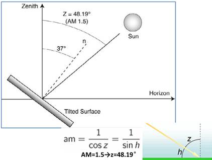
Below is my own sketch of the AM1.5G geometry (absorber is a plane tilted at 37°, with AM1.5 irradiation) created with TikZ (all angles are correct, but lengths are only illustrative):
caption.am15g.geometry <- paste( "The AM1.5G spectrum of the G173-03 ASTM reference is based on a receiving surface", "at an inclined plane at a tilt angle of 37° towards the equator and facing the sun", "at a zenith angle of 48.2° (air mass 1.5),", "with atmospheric conditions based on the 1976 U.S. Standard Atmosphere.") knitr::include_graphics(here("man/figures/AM15G-geometry.png"))
At air mass 1.5 the zenith angle is 48.2°, and the solar altitude is (the complementary angle) 41.8°. Note how the tilted absorber negates some of the projection effect (in the sketch, the tilted plane absorbs six solar rays, whereas the horizontal plane absorbs only five). That is, of course, the whole point of tilting the absorbing surface at higher altitudes. 37° roughly matches the average latitude of the contiguous United States, and air mass 1.5, as we have seen, corresponds to a latitude of 48° which is representative of the temperate zone wherein many industrialised cities around the world happen to be located.
Sources
- https://www.nrel.gov/grid/solar-resource/spectra-am1.5.html
- https://en.wikipedia.org/w/index.php?title=Air_mass_(solar_energy)&oldid=1158991725
- https://en.wikipedia.org/w/index.php?title=Geographic_center_of_the_United_States&oldid=1159819200#Contiguous_United_States
- https://www.nrel.gov/grid/solar-resource/spectra-am1.5.html
R Package Documentation
Browse R Packages
We want your feedback!
Note that we can't provide technical support on individual packages. You should contact the package authors for that.
Embedding an R snippet on your website
Add the following code to your website.
For more information on customizing the embed code, read Embedding Snippets.