README.md
In dieghernan/tidyterra: 'tidyverse' Methods and 'ggplot2' Helpers for 'terra' Objects
tidyterra 


The goal of tidyterra is to provide common methods of the
tidyverse packages for
objects created with the
terra package:
SpatRaster and SpatVector. It also provides geoms for plotting
these objects with ggplot2.
Please cite tidyterra as:
Hernangómez, D., (2023). Using the tidyverse with terra objects: the
tidyterra package. Journal of Open Source Software, 8(91), 5751,
https://doi.org/10.21105/joss.05751.
A BibTeX entry for LaTeX users is:
@article{Hernangómez2023,
  doi = {10.21105/joss.05751},
  url = {https://doi.org/10.21105/joss.05751},
  year = {2023},
  publisher = {The Open Journal},
  volume = {8},
  number = {91},
  pages = {5751},
  author = {Diego Hernangómez},
  title = {Using the {tidyverse} with {terra} objects: the {tidyterra} package},
  journal = {Journal of Open Source Software}
}
Overview
Full manual of the most recent release of tidyterra on CRAN is
online: https://dieghernan.github.io/tidyterra/
tidyverse methods implemented on tidyterra works differently
depending on the type of Spat* object:
-
SpatVector: the methods are implemented using
terra::as.data.frame() coercion. Rows correspond to geometries and
columns correspond to attributes of the geometry.
-
SpatRaster: The implementation on SpatRaster objects differs,
since the methods could be applied to layers or to cells.
tidyterra overall approach is to treat the layers as columns of a
tibble and the cells as rows (i.e. select(SpatRaster, 1) would
select the first layer of a SpatRaster).
The methods implemented return the same type of object used as input,
unless the expected behavior of the method is to return another type of
object, (for example, as_tibble() would return a tibble).
Current methods and functions provided by tidyterra are:
| tidyverse method | SpatVector | SpatRaster |
|----|----|----|
| tibble::as_tibble() | ✔️ | ✔️ |
| dplyr::select() | ✔️ | ✔️ Select layers |
| dplyr::mutate() | ✔️ | ✔️ Create /modify layers |
| dplyr::transmute() | ✔️ | ✔️ |
| dplyr::filter() | ✔️ | ✔️ Modify cells values and (additionally) remove outer cells. |
| dplyr::slice() | ✔️ | ✔️ Additional methods for slicing by row and column. |
| dplyr::pull() | ✔️ | ✔️ |
| dplyr::rename() | ✔️ | ✔️ |
| dplyr::relocate() | ✔️ | ✔️ |
| dplyr::distinct() | ✔️ | |
| dplyr::arrange() | ✔️ | |
| dplyr::glimpse() | ✔️ | ✔️ |
| dplyr::inner_join() family | ✔️ | |
| dplyr::summarise() | ✔️ | |
| dplyr::group_by() family | ✔️ | |
| dplyr::rowwise() | ✔️ | |
| dplyr::count(), tally() | ✔️ | |
| dplyr::bind_cols() / dplyr::bind_rows() | ✔️ as bind_spat_cols() / bind_spat_rows() | |
| tidyr::drop_na() | ✔️ | ✔️ Remove cell values with NA on any layer. Additionally, outer cells with NA are removed. |
| tidyr::replace_na() | ✔️ | ✔️ |
| tidyr::fill() | ✔️ | |
| tidyr::pivot_longer() | ✔️ | |
| tidyr::pivot_wider() | ✔️ | |
| ggplot2::autoplot() | ✔️ | ✔️ |
| ggplot2::fortify() | ✔️ to sf via sf::st_as_sf() | To a tibble with coordinates. |
| ggplot2::geom_*() | ✔️ geom_spatvector() | ✔️ geom_spatraster() and geom_spatraster_rgb(). |
:exclamation: A note on performance
tidyterra is conceived as a user-friendly wrapper of terra using
the tidyverse methods and verbs. This approach therefore has a
cost in terms of performance.
If you are a heavy user of terra or you need to work with big
raster files, terra is much more focused on terms of performance.
When possible, each function of tidyterra references to its
equivalent on terra.
As a rule of thumb if your raster has less than 10.000.000 data slots
counting cells and layers
(i.e. terra::ncell(your_rast)*terra::nlyr(your_rast) < 10e6) you are
good to go with tidyterra.
When plotting rasters, resampling is performed automatically (as
terra::plot() does, see the help page). You can adjust this with the
maxcell parameter.
Installation
Install tidyterra from
CRAN:
install.packages("tidyterra")
You can install the development version of tidyterra like so:
# install.packages("pak")
pak::pak("dieghernan/tidyterra")
Alternatively, you can install tidyterra using the
r-universe:
# Enable this universe
install.packages("tidyterra", repos = c(
  "https://dieghernan.r-universe.dev",
  "https://cloud.r-project.org"
))
Example
SpatRasters
This is a basic example which shows you how to manipulate and plot
SpatRaster objects:
library(tidyterra)
library(terra)
# Temperatures
rastertemp <- rast(system.file("extdata/cyl_temp.tif", package = "tidyterra"))
rastertemp
#> class : SpatRaster
#> size : 87, 118, 3 (nrow, ncol, nlyr)
#> resolution : 3881.255, 3881.255 (x, y)
#> extent : -612335.4, -154347.3, 4283018, 4620687 (xmin, xmax, ymin, ymax)
#> coord. ref. : World_Robinson
#> source : cyl_temp.tif
#> names : tavg_04, tavg_05, tavg_06
#> min values : 1.885463, 5.817587, 10.46338
#> max values : 13.283829, 16.740898, 21.11378
# Rename
rastertemp <- rastertemp %>%
rename(April = tavg_04, May = tavg_05, June = tavg_06)
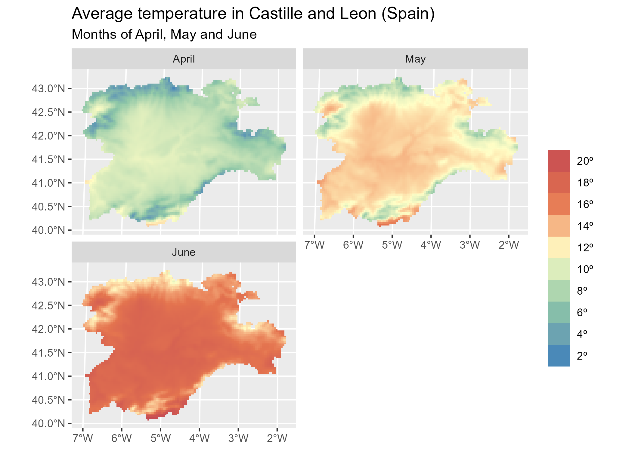
# Facet all layers
library(ggplot2)
ggplot() +
geom_spatraster(data = rastertemp) +
facet_wrap(~lyr, ncol = 2) +
scale_fill_whitebox_c(
palette = "muted",
labels = scales::label_number(suffix = "º"),
n.breaks = 12,
guide = guide_legend(reverse = TRUE)
) +
labs(
fill = "",
title = "Average temperature in Castille and Leon (Spain)",
subtitle = "Months of April, May and June"
)
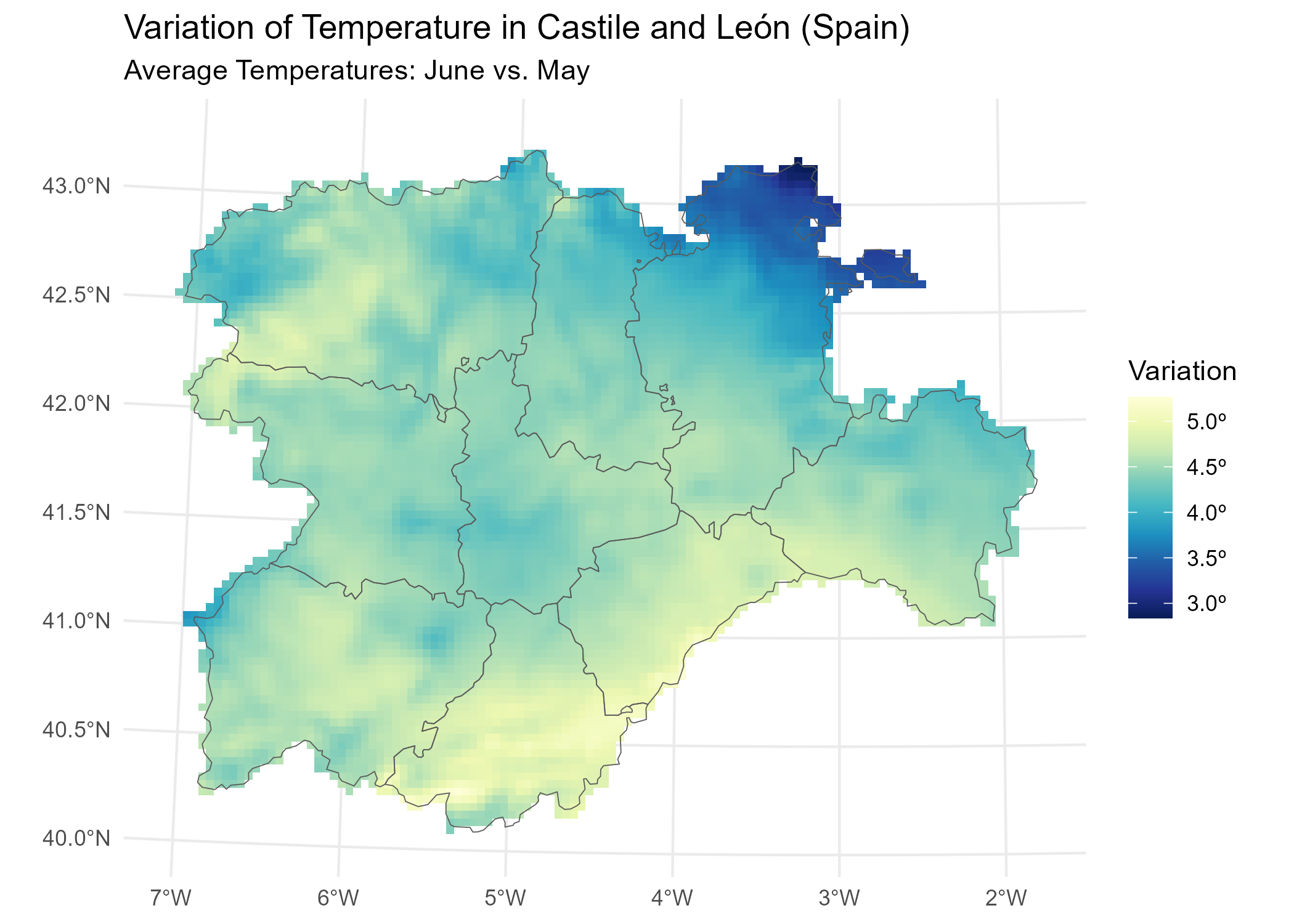
# Create maximum differences of two months
variation <- rastertemp %>%
  mutate(diff = June - May) %>%
  select(variation = diff)

# Add also a overlay of a SpatVector
prov <- vect(system.file("extdata/cyl.gpkg", package = "tidyterra"))

ggplot(prov) +
  geom_spatraster(data = variation) +
  geom_spatvector(fill = NA) +
  scale_fill_whitebox_c(
    palette = "deep", direction = -1,
    labels = scales::label_number(suffix = "º"),
    n.breaks = 5
  ) +
  theme_minimal() +
  coord_sf(crs = 25830) +
  labs(
    fill = "Variation",
    title = "Variation of Temperature in Castile and León (Spain)",
    subtitle = "Average Temperatures: June vs. May"
  )
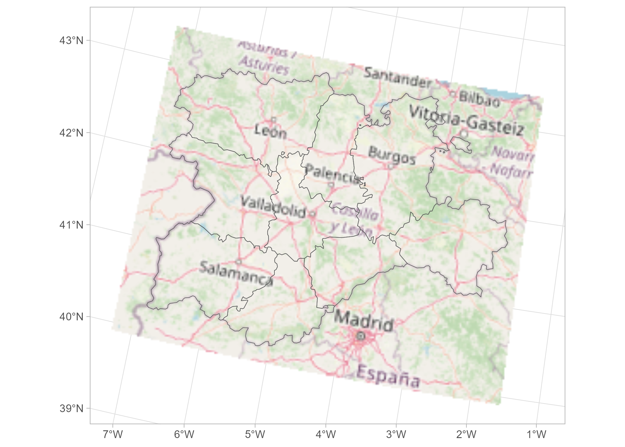
tidyterra also provides a geom for plotting RGB SpatRaster tiles
with ggplot2:
rgb_tile <- rast(system.file("extdata/cyl_tile.tif", package = "tidyterra"))

plot <- ggplot(prov) +
  geom_spatraster_rgb(data = rgb_tile) +
  geom_spatvector(fill = NA) +
  theme_light()

plot
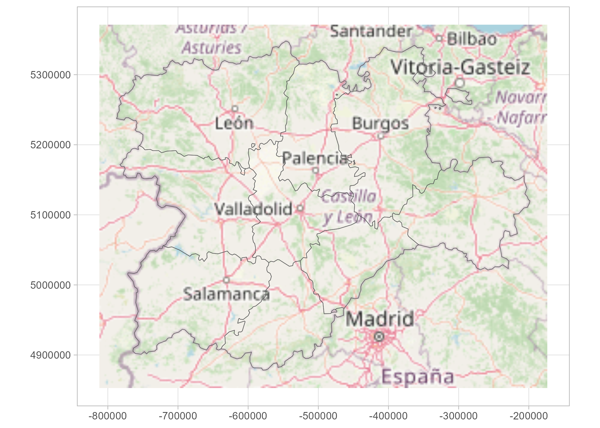
# Automatically recognizes and applies coord_sf() for spatial data.
plot +
  # Change the CRS and datum (useful for relabeling graticules).
  coord_sf(crs = 3857, datum = 3857)
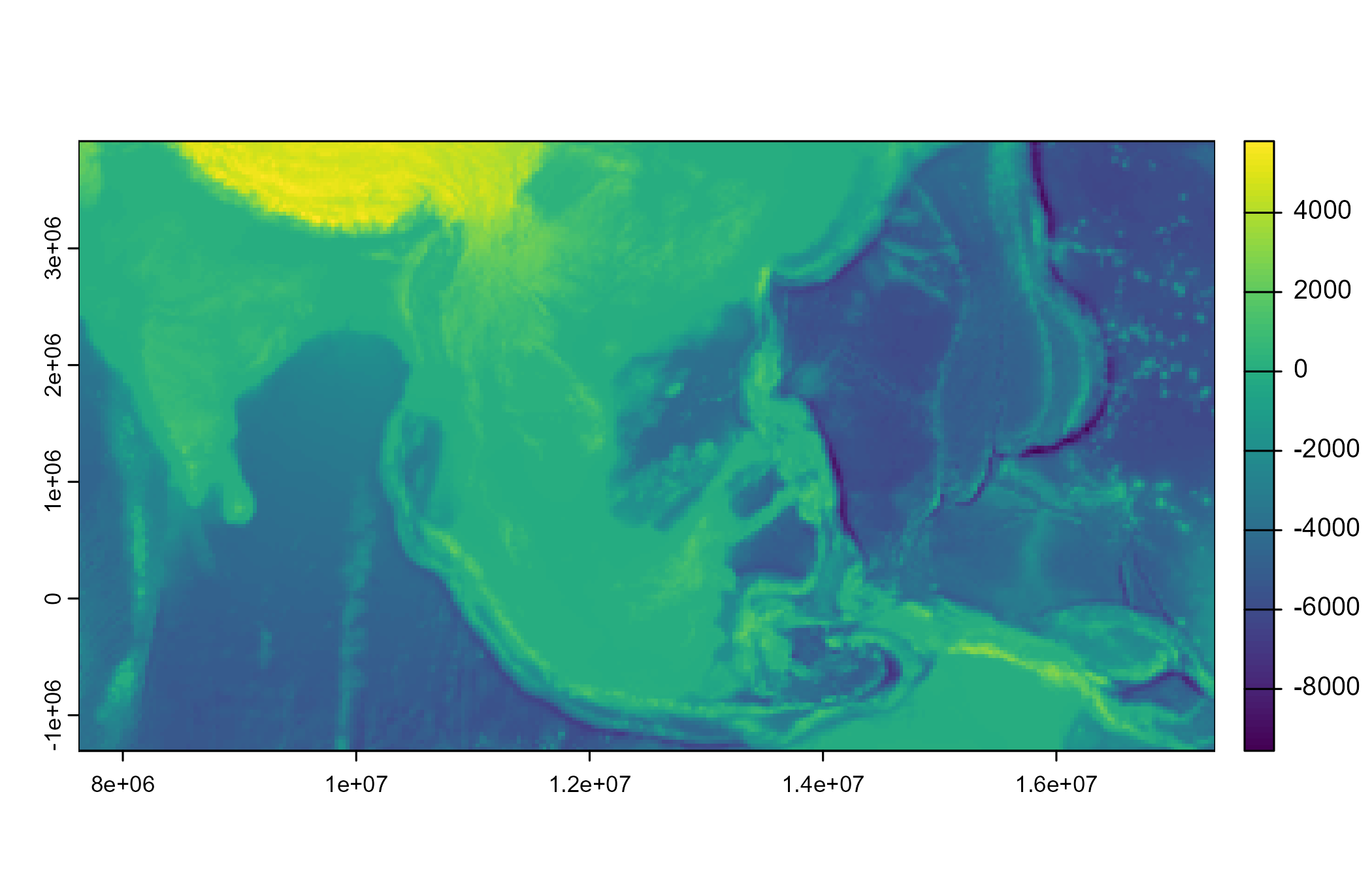
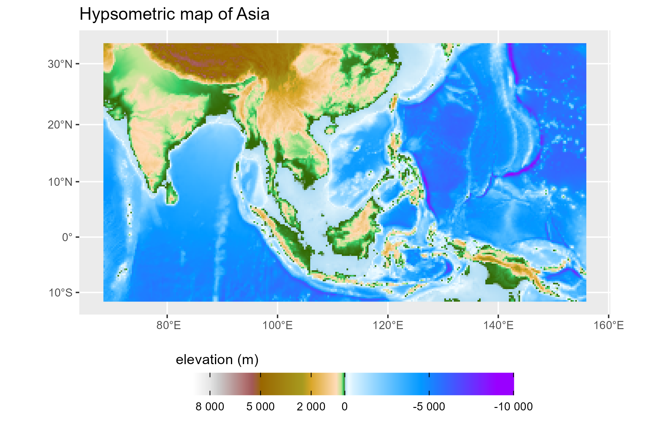
tidyterra provides specific scales for plotting hypsometric maps
with ggplot2:
asia <- rast(system.file("extdata/asia.tif", package = "tidyterra"))

terra::plot(asia)
ggplot() +
  geom_spatraster(data = asia) +
  scale_fill_hypso_tint_c(
    palette = "gmt_globe",
    labels = scales::label_number(),
    # Further refinements
    breaks = c(-10000, -5000, 0, 2000, 5000, 8000),
    guide = guide_colorbar(reverse = TRUE)
  ) +
  labs(
    fill = "elevation (m)",
    title = "Hypsometric map of Asia"
  ) +
  theme(
    legend.position = "bottom",
    legend.title.position = "top",
    legend.key.width = rel(3),
    legend.ticks = element_line(colour = "black", linewidth = 0.3),
    legend.direction = "horizontal"
  )
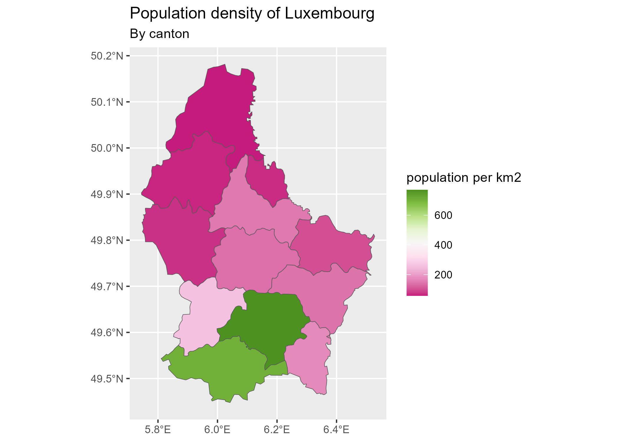
SpatVectors
This is a basic example which shows you how to manipulate and plot
SpatVector objects:
vect(system.file("ex/lux.shp", package = "terra")) %>%
  mutate(pop_dens = POP / AREA) %>%
  glimpse() %>%
  autoplot(aes(fill = pop_dens)) +
  scale_fill_whitebox_c(palette = "pi_y_g") +
  labs(
    fill = "population per km2",
    title = "Population density of Luxembourg",
    subtitle = "By canton"
  )
#> #  A SpatVector 12 x 7
#> #  Geometry type: Polygons
#> #  Geodetic CRS: lon/lat WGS 84 (EPSG:4326)
#> #  Extent (x / y) : ([5° 44' 38.9" E / 6° 31' 41.71" E] , [49° 26' 52.11" N / 50° 10' 53.84" N])
#>
#> $ ID_1     <dbl> 1, 1, 1, 1, 1, 2, 2, 2, 3, 3, 3, 3
#> $ NAME_1   <chr> "Diekirch", "Diekirch", "Diekirch", "Diekirch", "Diekirch", "…
#> $ ID_2     <dbl> 1, 2, 3, 4, 5, 6, 7, 12, 8, 9, 10, 11
#> $ NAME_2   <chr> "Clervaux", "Diekirch", "Redange", "Vianden", "Wiltz", "Echte…
#> $ AREA     <dbl> 312, 218, 259, 76, 263, 188, 129, 210, 185, 251, 237, 233
#> $ POP      <dbl> 18081, 32543, 18664, 5163, 16735, 18899, 22366, 29828, 48187,…
#> $ pop_dens <dbl> 57.95192, 149.27982, 72.06178, 67.93421, 63.63118, 100.52660,…
I need your feedback
Please leave your feedback or open an issue on
https://github.com/dieghernan/tidyterra/issues.
Need help?
Check our
FAQs or
open a new issue!
You can also ask in Stack Overflow using
the tag
[tidyterra].
Acknowledgement
tidyterra ggplot2 geoms are based on
ggspatial
implementation, by Dewey Dunnington
and ggspatial
contributors.
dieghernan/tidyterra documentation built on June 13, 2025, 6:02 p.m.
R Package Documentation
Browse R Packages
We want your feedback!
Note that we can't provide technical support on individual packages. You should contact the package authors for that.
tidyterra
![]()
![]()
![]()
![]()
![]()
![]()
![]()
The goal of tidyterra is to provide common methods of the
tidyverse packages for
objects created with the
terra package:
SpatRaster and SpatVector. It also provides geoms for plotting
these objects with ggplot2.
Please cite tidyterra as:
Hernangómez, D., (2023). Using the tidyverse with terra objects: the tidyterra package. Journal of Open Source Software, 8(91), 5751, https://doi.org/10.21105/joss.05751.
A BibTeX entry for LaTeX users is:
@article{Hernangómez2023,
doi = {10.21105/joss.05751},
url = {https://doi.org/10.21105/joss.05751},
year = {2023},
publisher = {The Open Journal},
volume = {8},
number = {91},
pages = {5751},
author = {Diego Hernangómez},
title = {Using the {tidyverse} with {terra} objects: the {tidyterra} package},
journal = {Journal of Open Source Software}
}
Overview
Full manual of the most recent release of tidyterra on CRAN is online: https://dieghernan.github.io/tidyterra/
tidyverse methods implemented on tidyterra works differently
depending on the type of Spat* object:
-
SpatVector: the methods are implemented usingterra::as.data.frame()coercion. Rows correspond to geometries and columns correspond to attributes of the geometry. -
SpatRaster: The implementation onSpatRasterobjects differs, since the methods could be applied to layers or to cells. tidyterra overall approach is to treat the layers as columns of a tibble and the cells as rows (i.e.select(SpatRaster, 1)would select the first layer of aSpatRaster).
The methods implemented return the same type of object used as input,
unless the expected behavior of the method is to return another type of
object, (for example, as_tibble() would return a tibble).
Current methods and functions provided by tidyterra are:
| tidyverse method | SpatVector | SpatRaster |
|----|----|----|
| tibble::as_tibble() | ✔️ | ✔️ |
| dplyr::select() | ✔️ | ✔️ Select layers |
| dplyr::mutate() | ✔️ | ✔️ Create /modify layers |
| dplyr::transmute() | ✔️ | ✔️ |
| dplyr::filter() | ✔️ | ✔️ Modify cells values and (additionally) remove outer cells. |
| dplyr::slice() | ✔️ | ✔️ Additional methods for slicing by row and column. |
| dplyr::pull() | ✔️ | ✔️ |
| dplyr::rename() | ✔️ | ✔️ |
| dplyr::relocate() | ✔️ | ✔️ |
| dplyr::distinct() | ✔️ | |
| dplyr::arrange() | ✔️ | |
| dplyr::glimpse() | ✔️ | ✔️ |
| dplyr::inner_join() family | ✔️ | |
| dplyr::summarise() | ✔️ | |
| dplyr::group_by() family | ✔️ | |
| dplyr::rowwise() | ✔️ | |
| dplyr::count(), tally() | ✔️ | |
| dplyr::bind_cols() / dplyr::bind_rows() | ✔️ as bind_spat_cols() / bind_spat_rows() | |
| tidyr::drop_na() | ✔️ | ✔️ Remove cell values with NA on any layer. Additionally, outer cells with NA are removed. |
| tidyr::replace_na() | ✔️ | ✔️ |
| tidyr::fill() | ✔️ | |
| tidyr::pivot_longer() | ✔️ | |
| tidyr::pivot_wider() | ✔️ | |
| ggplot2::autoplot() | ✔️ | ✔️ |
| ggplot2::fortify() | ✔️ to sf via sf::st_as_sf() | To a tibble with coordinates. |
| ggplot2::geom_*() | ✔️ geom_spatvector() | ✔️ geom_spatraster() and geom_spatraster_rgb(). |
:exclamation: A note on performance
tidyterra is conceived as a user-friendly wrapper of terra using the tidyverse methods and verbs. This approach therefore has a cost in terms of performance.
If you are a heavy user of terra or you need to work with big raster files, terra is much more focused on terms of performance. When possible, each function of tidyterra references to its equivalent on terra.
As a rule of thumb if your raster has less than 10.000.000 data slots
counting cells and layers
(i.e. terra::ncell(your_rast)*terra::nlyr(your_rast) < 10e6) you are
good to go with tidyterra.
When plotting rasters, resampling is performed automatically (as
terra::plot() does, see the help page). You can adjust this with the
maxcell parameter.
Installation
Install tidyterra from CRAN:
install.packages("tidyterra")
You can install the development version of tidyterra like so:
# install.packages("pak")
pak::pak("dieghernan/tidyterra")
Alternatively, you can install tidyterra using the r-universe:
# Enable this universe
install.packages("tidyterra", repos = c(
"https://dieghernan.r-universe.dev",
"https://cloud.r-project.org"
))
Example
SpatRasters
This is a basic example which shows you how to manipulate and plot
SpatRaster objects:
library(tidyterra)
library(terra)
# Temperatures
rastertemp <- rast(system.file("extdata/cyl_temp.tif", package = "tidyterra"))
rastertemp
#> class : SpatRaster
#> size : 87, 118, 3 (nrow, ncol, nlyr)
#> resolution : 3881.255, 3881.255 (x, y)
#> extent : -612335.4, -154347.3, 4283018, 4620687 (xmin, xmax, ymin, ymax)
#> coord. ref. : World_Robinson
#> source : cyl_temp.tif
#> names : tavg_04, tavg_05, tavg_06
#> min values : 1.885463, 5.817587, 10.46338
#> max values : 13.283829, 16.740898, 21.11378
# Rename
rastertemp <- rastertemp %>%
rename(April = tavg_04, May = tavg_05, June = tavg_06)
# Facet all layers
library(ggplot2)
ggplot() +
geom_spatraster(data = rastertemp) +
facet_wrap(~lyr, ncol = 2) +
scale_fill_whitebox_c(
palette = "muted",
labels = scales::label_number(suffix = "º"),
n.breaks = 12,
guide = guide_legend(reverse = TRUE)
) +
labs(
fill = "",
title = "Average temperature in Castille and Leon (Spain)",
subtitle = "Months of April, May and June"
)
# Create maximum differences of two months
variation <- rastertemp %>%
mutate(diff = June - May) %>%
select(variation = diff)
# Add also a overlay of a SpatVector
prov <- vect(system.file("extdata/cyl.gpkg", package = "tidyterra"))
ggplot(prov) +
geom_spatraster(data = variation) +
geom_spatvector(fill = NA) +
scale_fill_whitebox_c(
palette = "deep", direction = -1,
labels = scales::label_number(suffix = "º"),
n.breaks = 5
) +
theme_minimal() +
coord_sf(crs = 25830) +
labs(
fill = "Variation",
title = "Variation of Temperature in Castile and León (Spain)",
subtitle = "Average Temperatures: June vs. May"
)
tidyterra also provides a geom for plotting RGB SpatRaster tiles
with ggplot2:
rgb_tile <- rast(system.file("extdata/cyl_tile.tif", package = "tidyterra"))
plot <- ggplot(prov) +
geom_spatraster_rgb(data = rgb_tile) +
geom_spatvector(fill = NA) +
theme_light()
plot
# Automatically recognizes and applies coord_sf() for spatial data.
plot +
# Change the CRS and datum (useful for relabeling graticules).
coord_sf(crs = 3857, datum = 3857)
tidyterra provides specific scales for plotting hypsometric maps with ggplot2:
asia <- rast(system.file("extdata/asia.tif", package = "tidyterra"))
terra::plot(asia)
ggplot() +
geom_spatraster(data = asia) +
scale_fill_hypso_tint_c(
palette = "gmt_globe",
labels = scales::label_number(),
# Further refinements
breaks = c(-10000, -5000, 0, 2000, 5000, 8000),
guide = guide_colorbar(reverse = TRUE)
) +
labs(
fill = "elevation (m)",
title = "Hypsometric map of Asia"
) +
theme(
legend.position = "bottom",
legend.title.position = "top",
legend.key.width = rel(3),
legend.ticks = element_line(colour = "black", linewidth = 0.3),
legend.direction = "horizontal"
)
SpatVectors
This is a basic example which shows you how to manipulate and plot
SpatVector objects:
vect(system.file("ex/lux.shp", package = "terra")) %>%
mutate(pop_dens = POP / AREA) %>%
glimpse() %>%
autoplot(aes(fill = pop_dens)) +
scale_fill_whitebox_c(palette = "pi_y_g") +
labs(
fill = "population per km2",
title = "Population density of Luxembourg",
subtitle = "By canton"
)
#> # A SpatVector 12 x 7
#> # Geometry type: Polygons
#> # Geodetic CRS: lon/lat WGS 84 (EPSG:4326)
#> # Extent (x / y) : ([5° 44' 38.9" E / 6° 31' 41.71" E] , [49° 26' 52.11" N / 50° 10' 53.84" N])
#>
#> $ ID_1 <dbl> 1, 1, 1, 1, 1, 2, 2, 2, 3, 3, 3, 3
#> $ NAME_1 <chr> "Diekirch", "Diekirch", "Diekirch", "Diekirch", "Diekirch", "…
#> $ ID_2 <dbl> 1, 2, 3, 4, 5, 6, 7, 12, 8, 9, 10, 11
#> $ NAME_2 <chr> "Clervaux", "Diekirch", "Redange", "Vianden", "Wiltz", "Echte…
#> $ AREA <dbl> 312, 218, 259, 76, 263, 188, 129, 210, 185, 251, 237, 233
#> $ POP <dbl> 18081, 32543, 18664, 5163, 16735, 18899, 22366, 29828, 48187,…
#> $ pop_dens <dbl> 57.95192, 149.27982, 72.06178, 67.93421, 63.63118, 100.52660,…
I need your feedback
Please leave your feedback or open an issue on https://github.com/dieghernan/tidyterra/issues.
Need help?
Check our FAQs or open a new issue!
You can also ask in Stack Overflow using the tag [tidyterra].
Acknowledgement
tidyterra ggplot2 geoms are based on ggspatial implementation, by Dewey Dunnington and ggspatial contributors.
R Package Documentation
Browse R Packages
We want your feedback!
Note that we can't provide technical support on individual packages. You should contact the package authors for that.
Embedding an R snippet on your website
Add the following code to your website.
For more information on customizing the embed code, read Embedding Snippets.