inst/doc/rERR.R
In fbr600/rERR: Excess Relative Risk Models
#' ---
#' title: ""
#' author: "Francesc Badia Roca"
#' date: "`r Sys.Date()`"
#' output: rmarkdown::html_vignette
#' vignette: >
#' %\VignetteIndexEntry{Vignette Title}
#' %\VignetteEngine{knitr::rmarkdown}
#' \usepackage[utf8]{inputenc}
#' ---
#' # rERR package
#'
#' fit Excess Relative Risk model
#'
#' * [Introduction](https://github.com/fbr600/rERR#introduction)
#' * [Installing](https://github.com/fbr600/rERR#installing)
#' * [Model Specification](https://github.com/fbr600/rERR#model-specification)
#' * [Latency period (lag) and exclusion](https://github.com/fbr600/rERR#latency-period-lag-and-exclusion)
#' * [Examples](https://github.com/fbr600/rERR#examples)
#' + [Using an event format data set as input cohort](https://github.com/fbr600/rERR#using-an-event-format-data-set-as-input-cohort)
#' + [Using a wide format data set as input cohort](https://github.com/fbr600/rERR#using-a-wide-format-data-set-as-input-cohort)
#' + [Save time in multi analysis of the same data set](https://github.com/fbr600/rERR#save-time-in-multi-analysis-of-the-same-data-set)
#' + [Using Categorical Exposure](https://github.com/fbr600/rERR#using-categorical-exposure)
#' + [Plot the partial log likelihood function](https://github.com/fbr600/rERR/blob/master/README.md#plot-the-partial-log-likelihood-function)
#'
#' ## Introduction
#'
#' In radiation epidemiology, ERR models are used to analyze dose-response relationships for event rate data.
#'
#' Usual approaches to the analysis of cohort and case control data often follow from risk-set sampling designs, where at each failure
#' time a new risk set is defined, including the index case and all the controls that were at risk at that time. That kind of sampling
#' designs are usually related to the
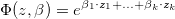
#' Cox proportional hazards model,
#'
#' 
#'
#' where  is the vector of explanatory variables,
#'
#' This model is available in most standard statistical packages but limited to log-linear model (except Epicure,(Preston et al., 1993)).
#'
#' One model of particular interest, especially in radiation environmental and occupational epidemiology is the linear ERR model,
#'
#' 
#'
#' where z is the vector of covariates.
#'
#' Estimation of a dose-response trend under a linear relative rate model implies that for every 1-unit increase in the exposure metric,
#' the rate of disease increases (or decreases) in an additive fashion.
#'
#' The modification of the effect of exposure in linear relative rate models by a study covariate z can be assessed by including a log-
#' linear subterm for the linear exposure, implying a model of the form
#'
#' 
#'
#' where  are the covariates.
#'
#' This package is an R impelementation of models that are rarely implemented outside Epicure: the Linear Excess Relative Risk model
#' allowing time dependent covariates, time dependent adjustments, lagged exposures and stratification.
#'
#' [back](https://github.com/fbr600/rERR/blob/master/README.md#rerr-package)
#'
#' ## Installing
#'
#' * With compilation of source code: it requires Rtools installed in your computer
#'
#' The package can be installed directly in RStudio from github:
#'
#' ```
#' install.packages("devtools")
#' devtools::install_github("fbr600/rERR")
#' ```
#' * Without compilation:
#'
#' You can download the .zip file [here](https://github.com/fbr600/rERR_binnary/raw/master/rERR.zip).
#'
#' Change the path to the download folder in the following code and run it in RStudio:
#'
#' ```
#' install.packages("path_to_downloads_folder/rERR.zip", repos = NULL, type = "win.binary")
#' install.packages("devtools")
#' devtools::install_deps(paste0(.libPaths(),"/rERR"))
#' ```
#' [back](https://github.com/fbr600/rERR/blob/master/README.md#rerr-package)
#'
#' ## Model Specification
#'
#' * The ERR model is specified using a formula object in R
#'
#' ```
#' formula <- Surv(entry_time,exit_time,outcome) ~ lin(dose_cum)
#' ```
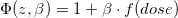
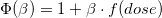
#' This is the formula for the model:
#'
#' 
#'
#' where f(dose) is the cumulative dose of each subject up to the relative fail time.
#'
#' * Also the covariates effect can be included in the model:
#' ```
#' formula <- Surv(entry_time,exit_time,outcome) ~ loglin(country) + lin(dose_cum)
#' ```
#' This is the formula of the model:
#'
#' 
#'
#' where  are the different countries.
#'
#' * Stratification in the risksets is done by using the ``` strata()``` function:
#' ```
#' formula <- Surv(entry_time,exit_time,outcome) ~ loglin(country) + lin(dose_cum) + strata(sex)
#' ```
#' Is the same model as before, but in the risksets only the subjects of the same sex as the case are taken as in-risk-subjects.
#'
#'
#' **Observation**
#' The data transformation required by the model computes the cumulative dose within the subject level over time, *dose_cum*, so this is a time-dependent variable, that is the cumulative dose recieved by each subject at every time.
#'
#' This variable always can be used as a variable, or can be used to recompute new variables such as other polynomic terms, cateogrizations of dose...
#'
#' [back](https://github.com/fbr600/rERR/blob/master/README.md#rerr-package)
#'
#' ## Latency period (lag) and exclusion
#'
#' The latency period is the estimated time after a certain exposure in which the dose-response is not possible.
#'
#' Analyzing the dose-response effect on a certain type of exposure, such as ionasing radiation, we want to exclude subjects that have a
#' failure or disease before that period because of misleading on causation.
#'
#' ##### Risk Model
#'
#' 
#'
#' So, imposing a latency period implies two actions:
#' * Remove subjects that have a follow-up shorter than lag period time
#' * Set the entry time to the cohort as 1st Exposure Time + lag , which is the moment in which a subject start being at risk
#'
#' [back](https://github.com/fbr600/rERR/blob/master/README.md#rerr-package)
#'
#' ## Examples
#' Two different formats of data sets are allowed:
#' * Event format data set (ef) - where each row represents an exposure event.
#' * Wide format data set (wf) - where each row contain all the follow-up information of a subject, icluding times and doses of exposures
#'
#' ### Using an event format data set as input cohort
#'
#' ##### load library
#' ```
#' > library(rERR)
#' ```
#' ##### look at the data set
#' ```
#' > head(cohort_ef,row.names=F)
#' id sex entry_age exit_age outcome age dose country
#' 10 2 9.88 12.53114 0 7.88 15.80825 Be
#' 14 1 11.09 12.35592 0 9.09 13.96742 UK
#' 14 1 11.09 12.35592 0 9.17 13.81423 UK
#' 15 1 9.55 12.33402 0 7.55 9.25016 Fr
#' 16 1 8.48 12.29843 0 6.49 18.00776 Sp
#' 16 1 8.48 12.29843 0 9.16 11.35068 Sp
#' ```
#'
#' ##### set the formulas for two models
#' ```
#' > formula1 <- Surv(entry_age,exit_age,outcome) ~ lin(dose_cum) + strata(sex)
#' > formula2 <- Surv(entry_age,exit_age,outcome) ~ loglin(factor(country)) + lin(dose_cum) + strata(sex)
#' ```
#'
#' ##### fit the models
#' ```
#' > fit1 <- f_fit_linERR_ef(formula1,data=cohort_ef,id_name="id",dose_name="dose",time_name="age",covars_names=c("sex"),lag=2,exclusion_done=T)
#' > fit2 <- f_fit_linERR_ef(formula2,data=cohort_ef,id_name="id",dose_name="dose",time_name="age",covars_names=c("sex","country"),lag=2,exclusion_done=T)
#' ```
#'
#' ##### summary of fit1
#' ```
#' > summary(fit1)
#' Formula:
#' Surv(entry_age, exit_age, outcome) ~ lin(dose_cum) + strata(sex)
#'
#' Linear Parameter Summary Table:
#' coef se(coef) z Pr(>|z|)
#' dose_cum 0.02401129 0.04400845 0.5456063 0.5853366
#'
#' AIC: 313.8759
#' Deviance: 311.8759
#' Number of risk sets: 18
#' ```
#'
#' ##### summary of fit2
#' ```
#' > summary(fit2)
#' Formula:
#' Surv(entry_age, exit_age, outcome) ~ loglin(factor(country)) +
#' lin(dose_cum) + strata(sex)
#'
#' Linear Parameter Summary Table:
#' coef se(coef) z Pr(>|z|)
#' dose_cum 0.02181835 0.04152847 0.5253829 0.5993171
#'
#' Log Linear Parameter Summary Table:
#' coef exp(coef) se(coef) z Pr(>|z|)
#' country_Fr 0.03444314 1.035043 1.0003142 0.03443232 0.9725324
#' country_Ge 0.70025564 2.014268 0.8660814 0.80853332 0.4187836
#' country_It 0.70146822 2.016712 0.8661484 0.80987072 0.4180145
#' country_Sp 0.04522023 1.046258 1.0001470 0.04521359 0.9639371
#' country_UK 0.69520396 2.004118 0.8661149 0.80266945 0.4221658
#'
#' AIC: 321.9591
#' Deviance: 309.9591
#' Number of risk sets: 18
#' ```
#'
#' ##### confidence intervals for fit1 parameters
#' ```
#' > confint(fit1)
#' Confidence intervals:
#'
#' Linear Parameter - Likelihood ratio test ci:
#' coef lower .95 upper .95
#' dose_cum 0.02401129 -0.01109805 0.8468688
#' ```
#'
#' ##### confidence intervals for fit2 parameters
#' ```
#' > confint(fit2)
#' Confidence intervals:
#'
#' Linear Parameter - Likelihood ratio test ci:
#' coef lower .95 upper .95
#' dose_cum 0.02181835 -0.01138425 0.774703
#'
#' Log Linear Parameter - Wald ci:
#' coef exp(coef) lower .95 upper .95
#' country_Fr 0.03444314 1.035043 0.1457101 7.352371
#' country_Ge 0.70025564 2.014268 0.3688989 10.998335
#' country_It 0.70146822 2.016712 0.3692980 11.013126
#' country_Sp 0.04522023 1.046258 0.1473371 7.429602
#' country_UK 0.69520396 2.004118 0.3670159 10.943634
#' ```
#'
#' ##### likelihood ratio test between nested and nesting models
#' ```
#' > f_lrt(fit1,fit2)
#' $lrt
#' [1] 1.916819
#'
#' $lrt_pval
#' [1] 0.3835023
#' ```
#' [back](https://github.com/fbr600/rERR/blob/master/README.md#rerr-package)
#'
#' ### Using a wide format data set as input cohort
#' ##### load library
#' ```
#' > library(rERR)
#' ```
#' ##### look at the data set
#' ```
#' > head(cohort_wf)
#' id sex YearInit AgeAtEntry age_at_event outcome end_status ses number_of_ct ctage1 ctage2 ... ctage35 dose1 dose2 ... dose35 country
#' 1 1 1983 7.957093 18.957093 0 2 1 1 7.957093 0 0 10.5 0 0 It
#' 2 1 1988 13.857040 18.857040 0 2 1 2 13.857040 0 0 10.4 0 0 Sp
#' 4 1 2008 16.496089 19.496089 0 2 1 1 16.496089 0 0 3.8 0 0 It
#' 12 1 2004 8.134463 17.134463 0 2 3 2 8.134463 0 0 7.0 0 0 Sp
#' 13 1 2009 2.554935 6.554935 0 2 2 2 2.554935 0 0 3.6 0 0 UK
#' 16 1 1996 16.968197 18.968197 0 2 3 1 16.968197 0 0 3.5 0 0 Fr
#' ```
#'
#' ##### set the formulas for the models
#' ```
#' > formula1 <- Surv(AgeAtEntry,age_at_event,outcome) ~ lin(dose_cum) + strata(sex)
#' > formula2 <- Surv(AgeAtEntry,age_at_event,outcome) ~ loglin(factor(country)) + lin(dose_cum) + strata(sex)
#' ```
#'
#' ##### fit the models
#' ```
#' > fit1 <- f_fit_linERR_wf(formula1,data=cohort_wf,id_name="id",doses=cohort_wf[,45:79],times=cohort_wf[,10:44],
#' covars=cohort_wf[,c("sex","country")],lag=2,exclusion_done = F)
#'
#' > fit2 <- f_fit_linERR_wf(formula2,data=cohort_wf,id_name="id",doses=cohort_wf[,45:79],times=cohort_wf[,10:44],
#' covars=cohort_wf[,c("sex","country")],lag=2,exclusion_done = F)
#' ```
#'
#' ##### summary of fit1
#' ```
#' > summary(fit1)
#' Formula:
#' Surv(AgeAtEntry, age_at_event, outcome) ~ lin(dose_cum) + strata(sex)
#'
#' Linear Parameter Summary Table:
#' coef se(coef) z Pr(>|z|)
#' dose_cum 0.03882416 0.03977917 0.975992 0.3290684
#'
#' AIC: 599.129
#' Deviance: 597.129
#' Number of risk sets: 34
#' ```
#' ##### summary of fit2
#' ```
#' > summary(fit2)
#' Formula:
#' Surv(AgeAtEntry, age_at_event, outcome) ~ loglin(factor(country)) +
#' lin(dose_cum) + strata(sex)
#'
#' Linear Parameter Summary Table:
#' coef se(coef) z Pr(>|z|)
#' dose_cum 0.0402001 0.04089224 0.9830742 0.3255709
#'
#' Log Linear Parameter Summary Table:
#' coef exp(coef) se(coef) z Pr(>|z|)
#' country_Fr -14.827568523 3.634702e-07 616.7428233 -0.02404174 0.9808193
#' country_Ge -0.005785829 9.942309e-01 0.5345654 -0.01082343 0.9913643
#' country_It 0.312718515 1.367137e+00 0.4929068 0.63443745 0.5257954
#' country_Sp -0.606014765 5.455206e-01 0.6268803 -0.96671535 0.3336864
#' country_UK -0.159932110 8.522016e-01 0.5565602 -0.28735816 0.7738381
#'
#' AIC: 593.5899
#' Deviance: 581.5899
#' Number of risk sets: 34
#' ```
#'
#' ##### confidence intervals for fit1 parameters
#' ```
#' > confint(fit1)
#' Confidence intervals:
#'
#' Linear Parameter - Likelihood ratio test ci:
#' coef lower .95 upper .95
#' dose_cum 0.03882416 -0.003425317 0.278199
#' ```
#'
#' ##### confidence intervals for fit2 parameters
#' ```
#' > confint(fit2)
#' Confidence intervals:
#'
#' Linear Parameter - Likelihood ratio test ci:
#' coef lower .95 upper .95
#' dose_cum 0.0402001 -0.003126192 0.2904963
#'
#' Log Linear Parameter - Wald ci:
#' coef exp(coef) lower .95 upper .95
#' country_Fr -14.827568523 3.634702e-07 0.0000000 Inf
#' country_Ge -0.005785829 9.942309e-01 0.3487100 2.834720
#' country_It 0.312718515 1.367137e+00 0.5202941 3.592319
#' country_Sp -0.606014765 5.455206e-01 0.1596650 1.863857
#' country_UK -0.159932110 8.522016e-01 0.2862843 2.536806
#' ```
#'
#' ##### likelihood ratio test between nested and nesting models
#' ```
#' > f_lrt(fit1,fit2)
#' $lrt
#' [1] 15.53904
#'
#' $lrt_pval
#' [1] 0.0004224168
#' ```
#'
#' [back](https://github.com/fbr600/rERR/blob/master/README.md#rerr-package)
#'
#' ### Save time in multi analysis of the same data set
#'
#' The process of fitting the model include an internal transformation of the data that can slow down the time of all process.
#'
#' Then if we need to run several analysis with the same data set, then we can run just one time the transfomation and run several
#' analysis on the transformed data set.
#'
#' The process can be splitted in three blocs:
#' * Do the exclusion
#' * Transform de data
#' * fit the model
#'
#' ```
#' f_fit_linERR_ef <- function (formula, data, id_name, dose_name, time_name, covars_names,lag,exclusion_done=F)
#' {
#' # exclude subjects with the follow-up shorter than lag (lattency period) time
#' if(!exclusion_done)
#' data <- f_exclusion(formula,data,lag)
#'
#' # this piece of code is encapsuled in the function: f_to_event_table_ef_all
#' {
#' form <- f_parse_formula(formula)
#' entry_name <- as.character(form$Surv$entry)
#' exit_name <- as.character(form$Surv$exit)
#' outcome_name <- as.character(form$Surv$outcome)
#' dt1 <- f_to_event_table_ef_v2(id = id_name, start = entry_name,
#' stop = exit_name, outcome = outcome_name, data = data,
#' doses = dose_name, times = time_name, covars = covars_names)
#' }
#'
#' # this piece of code is encapsuled in the function: f_fit_linERR_all
#' {
#' dt2 <- f_to_model_data(formula, data=dt1, id_name, time_name)
#' n_lin_vars <- attr(dt2, "n_lin_vars")
#' n_loglin_vars <- attr(dt2, "n_loglin_vars")
#' rsets <- f_risksets(formula, data = dt2, lag, id_name, time_name)
#' fit <- f_fit_linERR(formula, data = dt2, rsets, n_lin_vars,
#' n_loglin_vars, id_name, time_name)
#' return(fit)
#' }
#' }
#' ```
#'
#' Then if the exclusion and the data transfomration are common in two analysis, we do not have to do it twice:
#' ```
#' # specify the models we want to run
#' > formula1 <- Surv(entry_age,exit_age,outcome) ~ lin(dose_cum) + strata(sex)
#' > formula2 <- Surv(entry_age,exit_age,outcome) ~ loglin(factor(country)) + lin(dose_cum) + strata(sex)
#'
#' # we only need to set the variables:
#' > data <- cohort_ef
#' > exclusion_done <- TRUE
#' > lag <- 2
#' > id_name <- "id"
#' > time_name <- "age"
#' > dose_name <- "dose"
#'
#' # do the exclusion if needed
#' > if (!exclusion_done)
#' data <- f_exclusion(formula, data, lag)
#'
#' # transform the data including all the covariates required in all analysis
#' > dt1 <- f_to_event_table_ef_all(formula=formula1,data=data,id_name,dose_name,
#' time_name,covars_names=c("sex","country"))
#'
#' # fit the first model
#' > fit1 <- f_fit_linERR_all(formula1,data=dt1,id_name,time_name)
#'
#' # fit the second model
#' > fit2 <- f_fit_linERR_all(formula2,data=dt1,id_name,time_name)
#' ```
#'
#' [back](https://github.com/fbr600/rERR/blob/master/README.md#rerr-package)
#'
#' ### Using Categorical Exposure
#'
#' Often we want to know how the risk evolves through levels of exposure, to do this we can create a categorization of the dose and then put this categories into the model in the loglinear part.
#'
#' To do this the whole process can be broken in three main steps:
#' * Do the first data transformation
#' * Compute the categories of exposure
#' * Fit the model, so run the optimization
#'
#' ##### Do the first transformation
#'
#' Set the formula for the transformation and for the further categorical model, take into account that *dose_cat* still not exist, later on will be created:
#'
#' ```
#' > formula <- Surv(entry_age,exit_age,outcome) ~ loglin(dose_cat)+strata(sex)
#' ```
#'
#' Then run the transormation part,
#' ```
#' > dt1 <- f_to_event_table_ef_all(formula,data = cohort_ef,id_name = "id",dose_name = "dose",
#' time_name = "age",covars_names = c("sex","country"))
#' ```
#'
#' Look at the new data set:
#' ```
#' > head(dt1)
#' # A tibble: 6 x 13
#' # Groups: id_ [3]
#' id sex entry_age exit_age outcome age dose country id_ n_pe dose_num dose_cum id1
#' <int> <int> <dbl> <dbl> <dbl> <dbl> <dbl> <chr> <int> <dbl> <dbl> <dbl> <int>
#' 1 10 2 9.88 12.5 0 7.88 15.8 Be 10 1 15.8 15.8 1
#' 2 10 2 9.88 12.5 0 12.5 0 Be 10 0 0 15.8 1
#' 3 14 1 11.1 12.4 0 9.09 14.0 UK 14 1 14.0 14.0 2
#' 4 14 1 11.1 12.4 0 9.17 13.8 UK 14 2 13.8 27.8 2
#' 5 14 1 11.1 12.4 0 12.4 0 UK 14 0 0 27.8 2
#' 6 15 1 9.55 12.3 0 7.55 9.25 Fr 15 1 9.25 9.25 3
#' ```
#'
#' ##### Compute the categories of exposure
#'
#' The variable that will be categorized is *dose_cum* which is the cumulative dose at time *age*.
#' To decide what are the more appropiate cutoffs for the exposure levels usually basic descriptives are used:
#'
#' ```
#' > summary(dt1$dose_cum)
#' > hist(log(dt1$dose_cum))
#' ```
#' **Observation**
#' More accurate cutoffs can be described if only look at the doses that will be involved in the model, so it would imply to just look at the doses of the subjects in the risksets at the relatives failtimes.
#'
#' After see the distributions of several sets of cutoffs, select the choice:
#'
#' ```
#' > dt1$dose_cat <- cut(dt1$dose_cum, breaks = c(0,5,10,25,100,1000), right=F )
#' > plyr::count(dt1$dose_cat)
#' x freq
#' 1 [0,5) 18455
#' 2 [5,10) 26262
#' 3 [10,25) 46838
#' 4 [25,100) 37005
#' 5 [100,1e+03) 7490
#' ````
#' Fit the model
#'
#' ```
#' > fit <- f_fit_linERR_all(formula,data=dt1,id_name = "id",time_name = "age",lag = 2)
#' > summary(fit)
#' Formula:
#' Surv(entry_age, exit_age, outcome) ~ loglin(dose_cat) + strata(sex)
#'
#' Log Linear Parameter Summary Table:
#' coef exp(coef) se(coef) z Pr(>|z|)
#' dose_cat_[5,10) -17.3175712 3.013522e-08 8388.608701 -0.002064415 0.9983528
#' dose_cat_[10,25) 0.7851632 2.192765e+00 1.094160 0.717594248 0.4730075
#' dose_cat_[25,100) 1.6628654 5.274403e+00 1.073705 1.548717024 0.1214498
#' dose_cat_[100,1e+03) -14.0343748 8.034308e-07 2372.656914 -0.005915046 0.9952805
#'
#' AIC: 305.9834
#' Deviance: 297.9834
#' Number of risk sets: 18
#' ```
#'
#' [back](https://github.com/fbr600/rERR/blob/master/README.md#rerr-package)
#'
#' ### Plot the partial log likelihood function
#'
#' There is an option to display the shape of the log likelihood function:
#'
#' ```
#' # set the formulas for the models
#' formula1 <- Surv(entry_age,exit_age,outcome) ~ lin(dose_cum) + strata(sex)
#'
#' # fit the model
#' fit1 <- f_fit_linERR_ef(formula1,data=cohort_ef,id_name="id",dose_name="dose",
#' time_name="age",covars_names=c("sex"),lag=2,exclusion_done=TRUE)
#'
#' # plot the partial loglikelihood function
#' f_plot_linERR_ef(fit1,formula1,data=cohort_ef,id_name="id",dose_name="dose",
#' time_name="age",covars_names=c("sex"),lag=2,exclusion_done=TRUE)
#' ```
#'
#' And it appears the following plot:
#'
#' 
#'
#' [back](https://github.com/fbr600/rERR/blob/master/README.md#rerr-package)
fbr600/rERR documentation built on May 7, 2019, 9:36 a.m.
R Package Documentation
Browse R Packages
We want your feedback!
Note that we can't provide technical support on individual packages. You should contact the package authors for that.
#' ---
#' title: ""
#' author: "Francesc Badia Roca"
#' date: "`r Sys.Date()`"
#' output: rmarkdown::html_vignette
#' vignette: >
#' %\VignetteIndexEntry{Vignette Title}
#' %\VignetteEngine{knitr::rmarkdown}
#' \usepackage[utf8]{inputenc}
#' ---
#' # rERR package
#'
#' fit Excess Relative Risk model
#'
#' * [Introduction](https://github.com/fbr600/rERR#introduction)
#' * [Installing](https://github.com/fbr600/rERR#installing)
#' * [Model Specification](https://github.com/fbr600/rERR#model-specification)
#' * [Latency period (lag) and exclusion](https://github.com/fbr600/rERR#latency-period-lag-and-exclusion)
#' * [Examples](https://github.com/fbr600/rERR#examples)
#' + [Using an event format data set as input cohort](https://github.com/fbr600/rERR#using-an-event-format-data-set-as-input-cohort)
#' + [Using a wide format data set as input cohort](https://github.com/fbr600/rERR#using-a-wide-format-data-set-as-input-cohort)
#' + [Save time in multi analysis of the same data set](https://github.com/fbr600/rERR#save-time-in-multi-analysis-of-the-same-data-set)
#' + [Using Categorical Exposure](https://github.com/fbr600/rERR#using-categorical-exposure)
#' + [Plot the partial log likelihood function](https://github.com/fbr600/rERR/blob/master/README.md#plot-the-partial-log-likelihood-function)
#'
#' ## Introduction
#'
#' In radiation epidemiology, ERR models are used to analyze dose-response relationships for event rate data.
#'
#' Usual approaches to the analysis of cohort and case control data often follow from risk-set sampling designs, where at each failure
#' time a new risk set is defined, including the index case and all the controls that were at risk at that time. That kind of sampling
#' designs are usually related to the
#' Cox proportional hazards model,
#'
#' 
#'
#' where  is the vector of explanatory variables,
#'
#' This model is available in most standard statistical packages but limited to log-linear model (except Epicure,(Preston et al., 1993)).
#'
#' One model of particular interest, especially in radiation environmental and occupational epidemiology is the linear ERR model,
#'
#' 
#'
#' where z is the vector of covariates.
#'
#' Estimation of a dose-response trend under a linear relative rate model implies that for every 1-unit increase in the exposure metric,
#' the rate of disease increases (or decreases) in an additive fashion.
#'
#' The modification of the effect of exposure in linear relative rate models by a study covariate z can be assessed by including a log-
#' linear subterm for the linear exposure, implying a model of the form
#'
#' 
#'
#' where  are the covariates.
#'
#' This package is an R impelementation of models that are rarely implemented outside Epicure: the Linear Excess Relative Risk model
#' allowing time dependent covariates, time dependent adjustments, lagged exposures and stratification.
#'
#' [back](https://github.com/fbr600/rERR/blob/master/README.md#rerr-package)
#'
#' ## Installing
#'
#' * With compilation of source code: it requires Rtools installed in your computer
#'
#' The package can be installed directly in RStudio from github:
#'
#' ```
#' install.packages("devtools")
#' devtools::install_github("fbr600/rERR")
#' ```
#' * Without compilation:
#'
#' You can download the .zip file [here](https://github.com/fbr600/rERR_binnary/raw/master/rERR.zip).
#'
#' Change the path to the download folder in the following code and run it in RStudio:
#'
#' ```
#' install.packages("path_to_downloads_folder/rERR.zip", repos = NULL, type = "win.binary")
#' install.packages("devtools")
#' devtools::install_deps(paste0(.libPaths(),"/rERR"))
#' ```
#' [back](https://github.com/fbr600/rERR/blob/master/README.md#rerr-package)
#'
#' ## Model Specification
#'
#' * The ERR model is specified using a formula object in R
#'
#' ```
#' formula <- Surv(entry_time,exit_time,outcome) ~ lin(dose_cum)
#' ```
#' This is the formula for the model:
#'
#' 
#'
#' where f(dose) is the cumulative dose of each subject up to the relative fail time.
#'
#' * Also the covariates effect can be included in the model:
#' ```
#' formula <- Surv(entry_time,exit_time,outcome) ~ loglin(country) + lin(dose_cum)
#' ```
#' This is the formula of the model:
#'
#' 
#'
#' where  are the different countries.
#'
#' * Stratification in the risksets is done by using the ``` strata()``` function:
#' ```
#' formula <- Surv(entry_time,exit_time,outcome) ~ loglin(country) + lin(dose_cum) + strata(sex)
#' ```
#' Is the same model as before, but in the risksets only the subjects of the same sex as the case are taken as in-risk-subjects.
#'
#'
#' **Observation**
#' The data transformation required by the model computes the cumulative dose within the subject level over time, *dose_cum*, so this is a time-dependent variable, that is the cumulative dose recieved by each subject at every time.
#'
#' This variable always can be used as a variable, or can be used to recompute new variables such as other polynomic terms, cateogrizations of dose...
#'
#' [back](https://github.com/fbr600/rERR/blob/master/README.md#rerr-package)
#'
#' ## Latency period (lag) and exclusion
#'
#' The latency period is the estimated time after a certain exposure in which the dose-response is not possible.
#'
#' Analyzing the dose-response effect on a certain type of exposure, such as ionasing radiation, we want to exclude subjects that have a
#' failure or disease before that period because of misleading on causation.
#'
#' ##### Risk Model
#'
#' 
#'
#' So, imposing a latency period implies two actions:
#' * Remove subjects that have a follow-up shorter than lag period time
#' * Set the entry time to the cohort as 1st Exposure Time + lag , which is the moment in which a subject start being at risk
#'
#' [back](https://github.com/fbr600/rERR/blob/master/README.md#rerr-package)
#'
#' ## Examples
#' Two different formats of data sets are allowed:
#' * Event format data set (ef) - where each row represents an exposure event.
#' * Wide format data set (wf) - where each row contain all the follow-up information of a subject, icluding times and doses of exposures
#'
#' ### Using an event format data set as input cohort
#'
#' ##### load library
#' ```
#' > library(rERR)
#' ```
#' ##### look at the data set
#' ```
#' > head(cohort_ef,row.names=F)
#' id sex entry_age exit_age outcome age dose country
#' 10 2 9.88 12.53114 0 7.88 15.80825 Be
#' 14 1 11.09 12.35592 0 9.09 13.96742 UK
#' 14 1 11.09 12.35592 0 9.17 13.81423 UK
#' 15 1 9.55 12.33402 0 7.55 9.25016 Fr
#' 16 1 8.48 12.29843 0 6.49 18.00776 Sp
#' 16 1 8.48 12.29843 0 9.16 11.35068 Sp
#' ```
#'
#' ##### set the formulas for two models
#' ```
#' > formula1 <- Surv(entry_age,exit_age,outcome) ~ lin(dose_cum) + strata(sex)
#' > formula2 <- Surv(entry_age,exit_age,outcome) ~ loglin(factor(country)) + lin(dose_cum) + strata(sex)
#' ```
#'
#' ##### fit the models
#' ```
#' > fit1 <- f_fit_linERR_ef(formula1,data=cohort_ef,id_name="id",dose_name="dose",time_name="age",covars_names=c("sex"),lag=2,exclusion_done=T)
#' > fit2 <- f_fit_linERR_ef(formula2,data=cohort_ef,id_name="id",dose_name="dose",time_name="age",covars_names=c("sex","country"),lag=2,exclusion_done=T)
#' ```
#'
#' ##### summary of fit1
#' ```
#' > summary(fit1)
#' Formula:
#' Surv(entry_age, exit_age, outcome) ~ lin(dose_cum) + strata(sex)
#'
#' Linear Parameter Summary Table:
#' coef se(coef) z Pr(>|z|)
#' dose_cum 0.02401129 0.04400845 0.5456063 0.5853366
#'
#' AIC: 313.8759
#' Deviance: 311.8759
#' Number of risk sets: 18
#' ```
#'
#' ##### summary of fit2
#' ```
#' > summary(fit2)
#' Formula:
#' Surv(entry_age, exit_age, outcome) ~ loglin(factor(country)) +
#' lin(dose_cum) + strata(sex)
#'
#' Linear Parameter Summary Table:
#' coef se(coef) z Pr(>|z|)
#' dose_cum 0.02181835 0.04152847 0.5253829 0.5993171
#'
#' Log Linear Parameter Summary Table:
#' coef exp(coef) se(coef) z Pr(>|z|)
#' country_Fr 0.03444314 1.035043 1.0003142 0.03443232 0.9725324
#' country_Ge 0.70025564 2.014268 0.8660814 0.80853332 0.4187836
#' country_It 0.70146822 2.016712 0.8661484 0.80987072 0.4180145
#' country_Sp 0.04522023 1.046258 1.0001470 0.04521359 0.9639371
#' country_UK 0.69520396 2.004118 0.8661149 0.80266945 0.4221658
#'
#' AIC: 321.9591
#' Deviance: 309.9591
#' Number of risk sets: 18
#' ```
#'
#' ##### confidence intervals for fit1 parameters
#' ```
#' > confint(fit1)
#' Confidence intervals:
#'
#' Linear Parameter - Likelihood ratio test ci:
#' coef lower .95 upper .95
#' dose_cum 0.02401129 -0.01109805 0.8468688
#' ```
#'
#' ##### confidence intervals for fit2 parameters
#' ```
#' > confint(fit2)
#' Confidence intervals:
#'
#' Linear Parameter - Likelihood ratio test ci:
#' coef lower .95 upper .95
#' dose_cum 0.02181835 -0.01138425 0.774703
#'
#' Log Linear Parameter - Wald ci:
#' coef exp(coef) lower .95 upper .95
#' country_Fr 0.03444314 1.035043 0.1457101 7.352371
#' country_Ge 0.70025564 2.014268 0.3688989 10.998335
#' country_It 0.70146822 2.016712 0.3692980 11.013126
#' country_Sp 0.04522023 1.046258 0.1473371 7.429602
#' country_UK 0.69520396 2.004118 0.3670159 10.943634
#' ```
#'
#' ##### likelihood ratio test between nested and nesting models
#' ```
#' > f_lrt(fit1,fit2)
#' $lrt
#' [1] 1.916819
#'
#' $lrt_pval
#' [1] 0.3835023
#' ```
#' [back](https://github.com/fbr600/rERR/blob/master/README.md#rerr-package)
#'
#' ### Using a wide format data set as input cohort
#' ##### load library
#' ```
#' > library(rERR)
#' ```
#' ##### look at the data set
#' ```
#' > head(cohort_wf)
#' id sex YearInit AgeAtEntry age_at_event outcome end_status ses number_of_ct ctage1 ctage2 ... ctage35 dose1 dose2 ... dose35 country
#' 1 1 1983 7.957093 18.957093 0 2 1 1 7.957093 0 0 10.5 0 0 It
#' 2 1 1988 13.857040 18.857040 0 2 1 2 13.857040 0 0 10.4 0 0 Sp
#' 4 1 2008 16.496089 19.496089 0 2 1 1 16.496089 0 0 3.8 0 0 It
#' 12 1 2004 8.134463 17.134463 0 2 3 2 8.134463 0 0 7.0 0 0 Sp
#' 13 1 2009 2.554935 6.554935 0 2 2 2 2.554935 0 0 3.6 0 0 UK
#' 16 1 1996 16.968197 18.968197 0 2 3 1 16.968197 0 0 3.5 0 0 Fr
#' ```
#'
#' ##### set the formulas for the models
#' ```
#' > formula1 <- Surv(AgeAtEntry,age_at_event,outcome) ~ lin(dose_cum) + strata(sex)
#' > formula2 <- Surv(AgeAtEntry,age_at_event,outcome) ~ loglin(factor(country)) + lin(dose_cum) + strata(sex)
#' ```
#'
#' ##### fit the models
#' ```
#' > fit1 <- f_fit_linERR_wf(formula1,data=cohort_wf,id_name="id",doses=cohort_wf[,45:79],times=cohort_wf[,10:44],
#' covars=cohort_wf[,c("sex","country")],lag=2,exclusion_done = F)
#'
#' > fit2 <- f_fit_linERR_wf(formula2,data=cohort_wf,id_name="id",doses=cohort_wf[,45:79],times=cohort_wf[,10:44],
#' covars=cohort_wf[,c("sex","country")],lag=2,exclusion_done = F)
#' ```
#'
#' ##### summary of fit1
#' ```
#' > summary(fit1)
#' Formula:
#' Surv(AgeAtEntry, age_at_event, outcome) ~ lin(dose_cum) + strata(sex)
#'
#' Linear Parameter Summary Table:
#' coef se(coef) z Pr(>|z|)
#' dose_cum 0.03882416 0.03977917 0.975992 0.3290684
#'
#' AIC: 599.129
#' Deviance: 597.129
#' Number of risk sets: 34
#' ```
#' ##### summary of fit2
#' ```
#' > summary(fit2)
#' Formula:
#' Surv(AgeAtEntry, age_at_event, outcome) ~ loglin(factor(country)) +
#' lin(dose_cum) + strata(sex)
#'
#' Linear Parameter Summary Table:
#' coef se(coef) z Pr(>|z|)
#' dose_cum 0.0402001 0.04089224 0.9830742 0.3255709
#'
#' Log Linear Parameter Summary Table:
#' coef exp(coef) se(coef) z Pr(>|z|)
#' country_Fr -14.827568523 3.634702e-07 616.7428233 -0.02404174 0.9808193
#' country_Ge -0.005785829 9.942309e-01 0.5345654 -0.01082343 0.9913643
#' country_It 0.312718515 1.367137e+00 0.4929068 0.63443745 0.5257954
#' country_Sp -0.606014765 5.455206e-01 0.6268803 -0.96671535 0.3336864
#' country_UK -0.159932110 8.522016e-01 0.5565602 -0.28735816 0.7738381
#'
#' AIC: 593.5899
#' Deviance: 581.5899
#' Number of risk sets: 34
#' ```
#'
#' ##### confidence intervals for fit1 parameters
#' ```
#' > confint(fit1)
#' Confidence intervals:
#'
#' Linear Parameter - Likelihood ratio test ci:
#' coef lower .95 upper .95
#' dose_cum 0.03882416 -0.003425317 0.278199
#' ```
#'
#' ##### confidence intervals for fit2 parameters
#' ```
#' > confint(fit2)
#' Confidence intervals:
#'
#' Linear Parameter - Likelihood ratio test ci:
#' coef lower .95 upper .95
#' dose_cum 0.0402001 -0.003126192 0.2904963
#'
#' Log Linear Parameter - Wald ci:
#' coef exp(coef) lower .95 upper .95
#' country_Fr -14.827568523 3.634702e-07 0.0000000 Inf
#' country_Ge -0.005785829 9.942309e-01 0.3487100 2.834720
#' country_It 0.312718515 1.367137e+00 0.5202941 3.592319
#' country_Sp -0.606014765 5.455206e-01 0.1596650 1.863857
#' country_UK -0.159932110 8.522016e-01 0.2862843 2.536806
#' ```
#'
#' ##### likelihood ratio test between nested and nesting models
#' ```
#' > f_lrt(fit1,fit2)
#' $lrt
#' [1] 15.53904
#'
#' $lrt_pval
#' [1] 0.0004224168
#' ```
#'
#' [back](https://github.com/fbr600/rERR/blob/master/README.md#rerr-package)
#'
#' ### Save time in multi analysis of the same data set
#'
#' The process of fitting the model include an internal transformation of the data that can slow down the time of all process.
#'
#' Then if we need to run several analysis with the same data set, then we can run just one time the transfomation and run several
#' analysis on the transformed data set.
#'
#' The process can be splitted in three blocs:
#' * Do the exclusion
#' * Transform de data
#' * fit the model
#'
#' ```
#' f_fit_linERR_ef <- function (formula, data, id_name, dose_name, time_name, covars_names,lag,exclusion_done=F)
#' {
#' # exclude subjects with the follow-up shorter than lag (lattency period) time
#' if(!exclusion_done)
#' data <- f_exclusion(formula,data,lag)
#'
#' # this piece of code is encapsuled in the function: f_to_event_table_ef_all
#' {
#' form <- f_parse_formula(formula)
#' entry_name <- as.character(form$Surv$entry)
#' exit_name <- as.character(form$Surv$exit)
#' outcome_name <- as.character(form$Surv$outcome)
#' dt1 <- f_to_event_table_ef_v2(id = id_name, start = entry_name,
#' stop = exit_name, outcome = outcome_name, data = data,
#' doses = dose_name, times = time_name, covars = covars_names)
#' }
#'
#' # this piece of code is encapsuled in the function: f_fit_linERR_all
#' {
#' dt2 <- f_to_model_data(formula, data=dt1, id_name, time_name)
#' n_lin_vars <- attr(dt2, "n_lin_vars")
#' n_loglin_vars <- attr(dt2, "n_loglin_vars")
#' rsets <- f_risksets(formula, data = dt2, lag, id_name, time_name)
#' fit <- f_fit_linERR(formula, data = dt2, rsets, n_lin_vars,
#' n_loglin_vars, id_name, time_name)
#' return(fit)
#' }
#' }
#' ```
#'
#' Then if the exclusion and the data transfomration are common in two analysis, we do not have to do it twice:
#' ```
#' # specify the models we want to run
#' > formula1 <- Surv(entry_age,exit_age,outcome) ~ lin(dose_cum) + strata(sex)
#' > formula2 <- Surv(entry_age,exit_age,outcome) ~ loglin(factor(country)) + lin(dose_cum) + strata(sex)
#'
#' # we only need to set the variables:
#' > data <- cohort_ef
#' > exclusion_done <- TRUE
#' > lag <- 2
#' > id_name <- "id"
#' > time_name <- "age"
#' > dose_name <- "dose"
#'
#' # do the exclusion if needed
#' > if (!exclusion_done)
#' data <- f_exclusion(formula, data, lag)
#'
#' # transform the data including all the covariates required in all analysis
#' > dt1 <- f_to_event_table_ef_all(formula=formula1,data=data,id_name,dose_name,
#' time_name,covars_names=c("sex","country"))
#'
#' # fit the first model
#' > fit1 <- f_fit_linERR_all(formula1,data=dt1,id_name,time_name)
#'
#' # fit the second model
#' > fit2 <- f_fit_linERR_all(formula2,data=dt1,id_name,time_name)
#' ```
#'
#' [back](https://github.com/fbr600/rERR/blob/master/README.md#rerr-package)
#'
#' ### Using Categorical Exposure
#'
#' Often we want to know how the risk evolves through levels of exposure, to do this we can create a categorization of the dose and then put this categories into the model in the loglinear part.
#'
#' To do this the whole process can be broken in three main steps:
#' * Do the first data transformation
#' * Compute the categories of exposure
#' * Fit the model, so run the optimization
#'
#' ##### Do the first transformation
#'
#' Set the formula for the transformation and for the further categorical model, take into account that *dose_cat* still not exist, later on will be created:
#'
#' ```
#' > formula <- Surv(entry_age,exit_age,outcome) ~ loglin(dose_cat)+strata(sex)
#' ```
#'
#' Then run the transormation part,
#' ```
#' > dt1 <- f_to_event_table_ef_all(formula,data = cohort_ef,id_name = "id",dose_name = "dose",
#' time_name = "age",covars_names = c("sex","country"))
#' ```
#'
#' Look at the new data set:
#' ```
#' > head(dt1)
#' # A tibble: 6 x 13
#' # Groups: id_ [3]
#' id sex entry_age exit_age outcome age dose country id_ n_pe dose_num dose_cum id1
#' <int> <int> <dbl> <dbl> <dbl> <dbl> <dbl> <chr> <int> <dbl> <dbl> <dbl> <int>
#' 1 10 2 9.88 12.5 0 7.88 15.8 Be 10 1 15.8 15.8 1
#' 2 10 2 9.88 12.5 0 12.5 0 Be 10 0 0 15.8 1
#' 3 14 1 11.1 12.4 0 9.09 14.0 UK 14 1 14.0 14.0 2
#' 4 14 1 11.1 12.4 0 9.17 13.8 UK 14 2 13.8 27.8 2
#' 5 14 1 11.1 12.4 0 12.4 0 UK 14 0 0 27.8 2
#' 6 15 1 9.55 12.3 0 7.55 9.25 Fr 15 1 9.25 9.25 3
#' ```
#'
#' ##### Compute the categories of exposure
#'
#' The variable that will be categorized is *dose_cum* which is the cumulative dose at time *age*.
#' To decide what are the more appropiate cutoffs for the exposure levels usually basic descriptives are used:
#'
#' ```
#' > summary(dt1$dose_cum)
#' > hist(log(dt1$dose_cum))
#' ```
#' **Observation**
#' More accurate cutoffs can be described if only look at the doses that will be involved in the model, so it would imply to just look at the doses of the subjects in the risksets at the relatives failtimes.
#'
#' After see the distributions of several sets of cutoffs, select the choice:
#'
#' ```
#' > dt1$dose_cat <- cut(dt1$dose_cum, breaks = c(0,5,10,25,100,1000), right=F )
#' > plyr::count(dt1$dose_cat)
#' x freq
#' 1 [0,5) 18455
#' 2 [5,10) 26262
#' 3 [10,25) 46838
#' 4 [25,100) 37005
#' 5 [100,1e+03) 7490
#' ````
#' Fit the model
#'
#' ```
#' > fit <- f_fit_linERR_all(formula,data=dt1,id_name = "id",time_name = "age",lag = 2)
#' > summary(fit)
#' Formula:
#' Surv(entry_age, exit_age, outcome) ~ loglin(dose_cat) + strata(sex)
#'
#' Log Linear Parameter Summary Table:
#' coef exp(coef) se(coef) z Pr(>|z|)
#' dose_cat_[5,10) -17.3175712 3.013522e-08 8388.608701 -0.002064415 0.9983528
#' dose_cat_[10,25) 0.7851632 2.192765e+00 1.094160 0.717594248 0.4730075
#' dose_cat_[25,100) 1.6628654 5.274403e+00 1.073705 1.548717024 0.1214498
#' dose_cat_[100,1e+03) -14.0343748 8.034308e-07 2372.656914 -0.005915046 0.9952805
#'
#' AIC: 305.9834
#' Deviance: 297.9834
#' Number of risk sets: 18
#' ```
#'
#' [back](https://github.com/fbr600/rERR/blob/master/README.md#rerr-package)
#'
#' ### Plot the partial log likelihood function
#'
#' There is an option to display the shape of the log likelihood function:
#'
#' ```
#' # set the formulas for the models
#' formula1 <- Surv(entry_age,exit_age,outcome) ~ lin(dose_cum) + strata(sex)
#'
#' # fit the model
#' fit1 <- f_fit_linERR_ef(formula1,data=cohort_ef,id_name="id",dose_name="dose",
#' time_name="age",covars_names=c("sex"),lag=2,exclusion_done=TRUE)
#'
#' # plot the partial loglikelihood function
#' f_plot_linERR_ef(fit1,formula1,data=cohort_ef,id_name="id",dose_name="dose",
#' time_name="age",covars_names=c("sex"),lag=2,exclusion_done=TRUE)
#' ```
#'
#' And it appears the following plot:
#'
#' 
#'
#' [back](https://github.com/fbr600/rERR/blob/master/README.md#rerr-package)
R Package Documentation
Browse R Packages
We want your feedback!
Note that we can't provide technical support on individual packages. You should contact the package authors for that.
Embedding an R snippet on your website
Add the following code to your website.
For more information on customizing the embed code, read Embedding Snippets.