README.md

In filipematias23/cleanRfield: A tool for cleaning and filtering data spatial points from agricultural field trials

cleanRfield: A tool for cleaning and filtering data spatial points from crop yield maps in R.

This package is a compilation of functions to clean and filter observations from yield monitors or other agricultural spatial point data. Yield monitors are prone to error, and filtering the observations or removing observations from near field boundaries can improve estimates of whole-field yield, combine speed, grain moisture, or other parameters of interest. In this package, users can easily select filters for one or more traits and prepare a smaller dataset to make decisions.

This tutorial assumes that readers have a basic understanding of spatial data, including projections and coordinate reference systems. If you need a refresher on this topic, we recommend reading this blog post for deciding between projected and unprojected data and this post for understanding the basics of coordinate reference systems.

--------------------------------------------- ## Resources [Installation](#instal) [1. First steps](#p1) [2. Cropping or selecting regions](#p2) [3. Sampling point data](#p3) [4. Making rasters](#p4) [5. Building shape boundaries](#p5) [6. Buffering the field boundaries](#p6) [7. Filtering using data values](#p7) [8. Filtering using standard deviation values](#p8) [9. Evaluating multiple fields on parallel](#p9) [10. Making Maps](#p10) [11. Saving files](#p11) [12. Working with .csv or .txt files](#p12) [13. Interpolating yield maps](#p13) [Contact](#pC)

--------------------------------------------- > Install [R](https://www.r-project.org/) and [RStudio](https://rstudio.com/). > Now install R/cleanRfield using the `install_github()` function from [devtools](https://github.com/hadley/devtools) package. If necessary, use the argument [*type="source"*](https://www.rdocumentation.org/packages/ghit/versions/0.2.18/topics/install_github). wzxhzdk:0

[Menu](#menu)

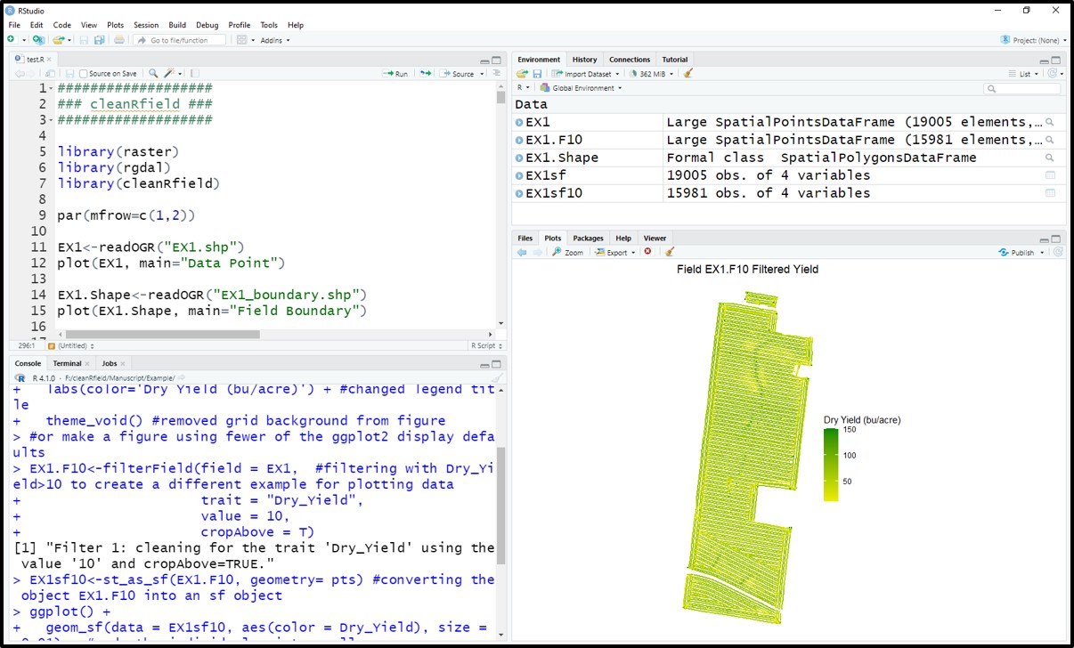
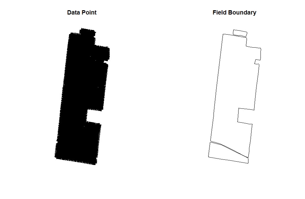
--------------------------------------------- #### 1. First steps > **Calling necessary packages:** wzxhzdk:1 > Start this tutorial by downloading the example EX1 [here](https://drive.google.com/file/d/1FTdbrp-_SE81vUoQv4wBsqVGqkUUUaPR/view?usp=sharing) and the field boundary [here](https://drive.google.com/file/d/1pP41HiG2RxF7HOu_5fdj6Pg9DoTaLPcy/view?usp=sharing). This tutorial will use the function *`vect()`* from package **terra** to read and upload the data to RStudio (see provided code). 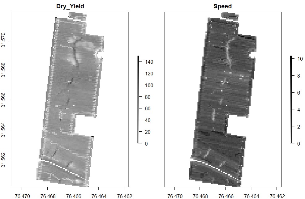> EX1 is a yield map from a soybean field, stored as a point shapefile. Yield monitor observations were originally collected in the north-central US using a combine yield monitor, and observations were geographically shifted to protect the landowner’s privacy. This data set include three attributes: > * Speed (miles per hour): speed of the combine at the time the observation was recorded > * Dry_Yield (bushels per acre): yield at that observation’s location as recorded by the yield monitor, adjusted to a 13% moisture basis > * Adj_Moist (percent): indicates what moisture level the original wet yield measurements were adjusted to when calculating dry yield > The field boundary is a shapefile layer with three (3) polygons that delineate the boundaries of the sample field EX1. wzxhzdk:2

[Menu](#menu)

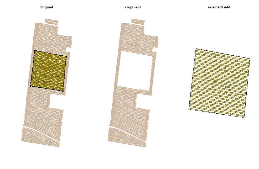
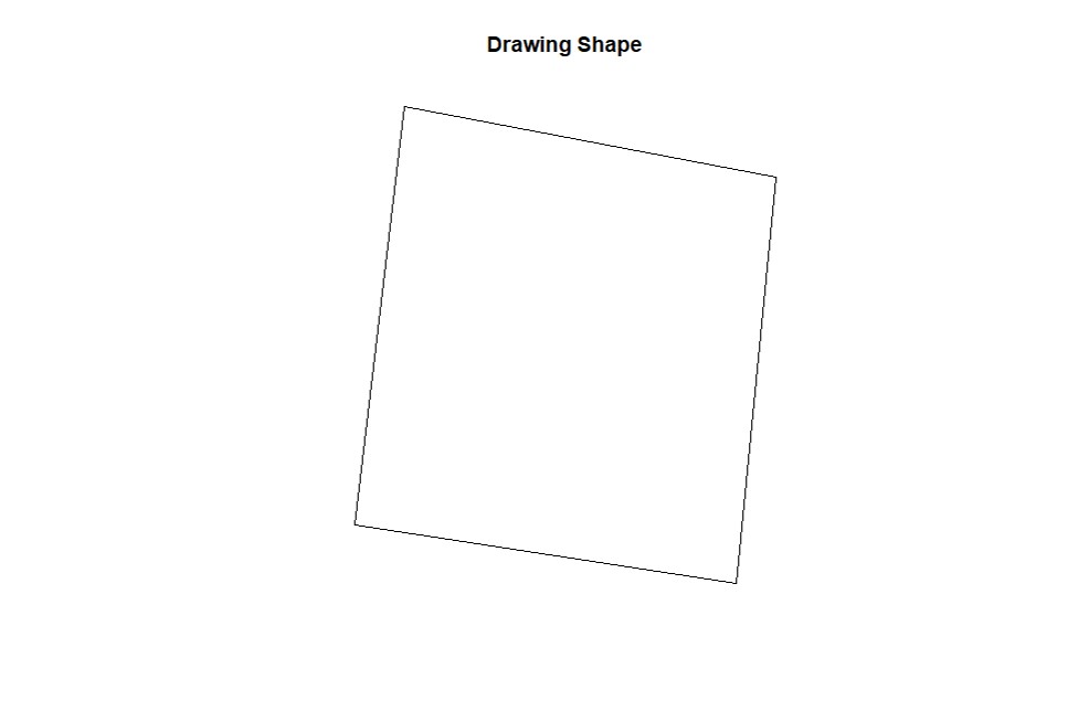
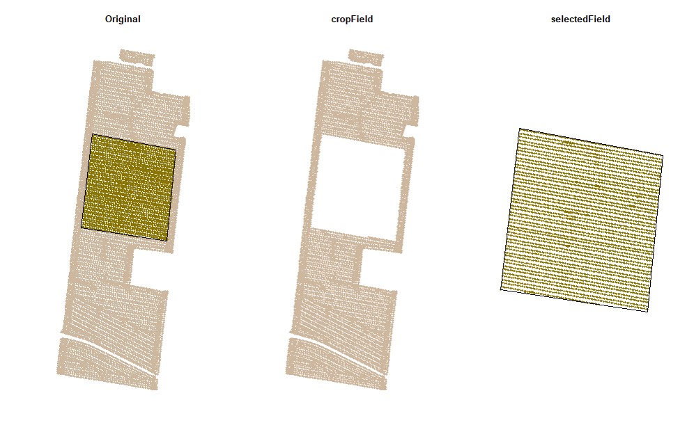
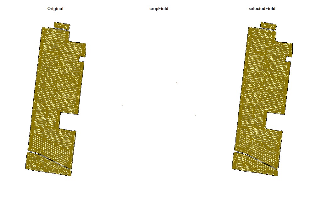
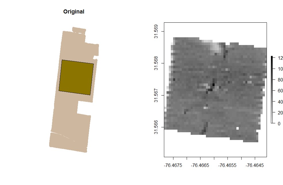
--------------------------------------------- #### 2. Cropping or selecting targeted field > Users can subset the data by drawing boundaries around a field or subset of fields. Function **`cropField`**. Depending on your computer and the size of your data set, this step may take a few seconds. This function works better using a popup window, not RStudio's integrated viewing pane, so we've included code for opening that new window. wzxhzdk:3

wzxhzdk:4

wzxhzdk:5

wzxhzdk:6

> The newest version of RStudio (2021.09.2) has updated the plot viewing pane. If you are using the newest RStudio, you may need run an additional line of code to open the point-and-click cropping functionality in a pop-out window instead of the integrated plot viewing pane. wzxhzdk:7 [Menu](#menu)

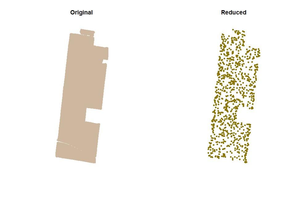
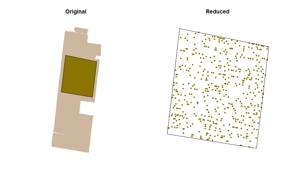
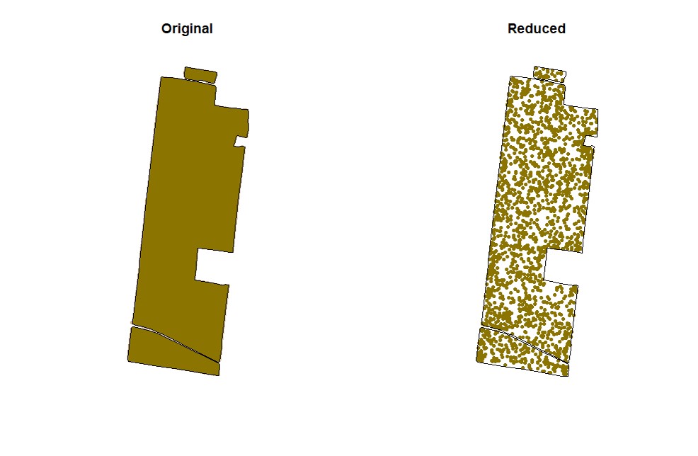
--------------------------------------------- #### 3. Sampling point data > Users can sample random points in the data. Function **`sampleField`**. wzxhzdk:8

wzxhzdk:9

wzxhzdk:10

[Menu](#menu)

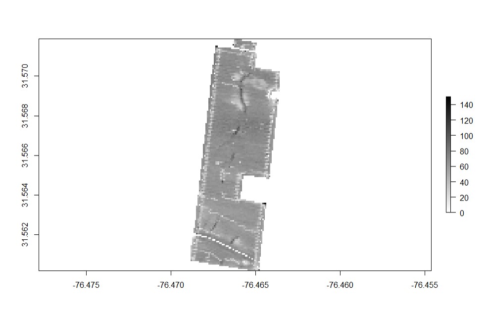
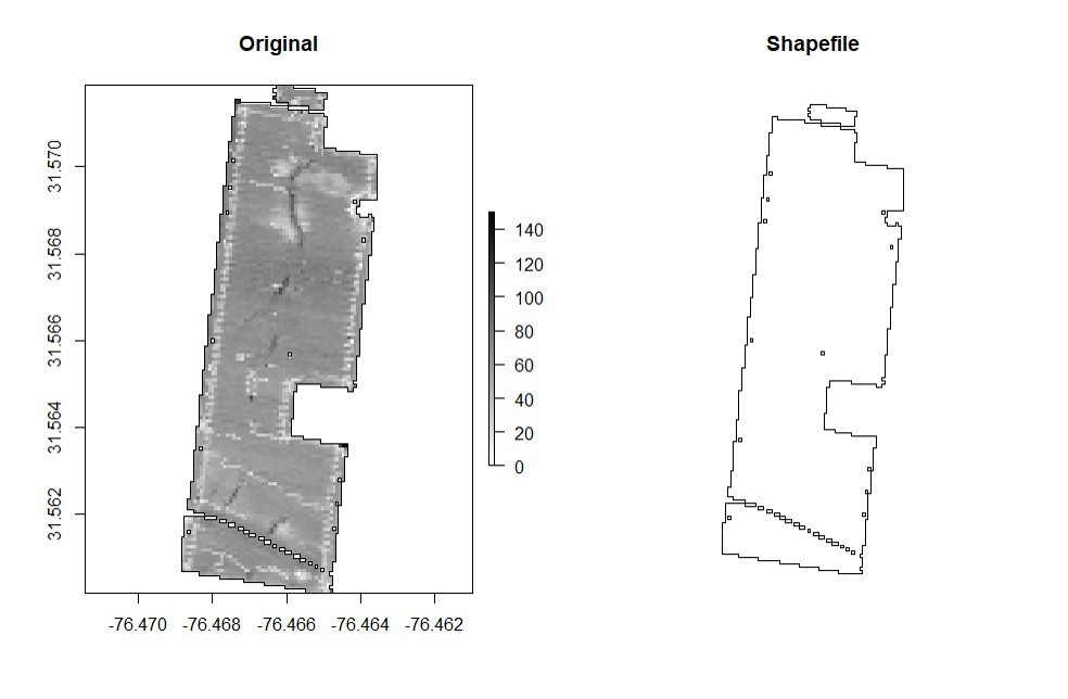
--------------------------------------------- #### 4. Making rasters > Function **`rasterField`**.Data points can be used to create raster files. Use either the provided code for unprojected data or projected data-- you will not need to run both sets of code. Any positive number can be chosen as the resolution, but choosing too high of a resolution will result in a raster file that oversimplifies the shape of the field, and choosing too low of a resolution can cause the runtime to be to long and/or cause the parts of the field between combine passes to be excluded from the final field shape. wzxhzdk:11

wzxhzdk:12

wzxhzdk:13

wzxhzdk:14

[Menu](#menu)

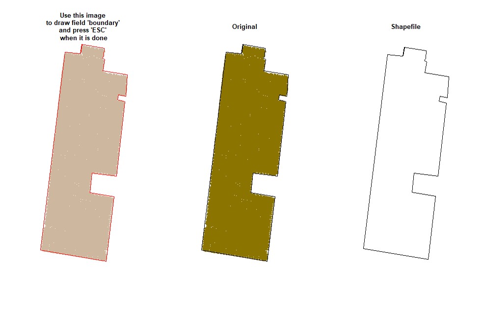
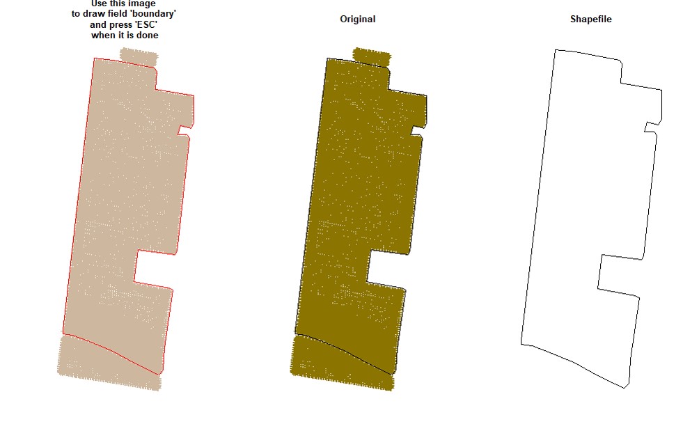
--------------------------------------------- #### 5. Building shape boundaries > Users can manually draw field boundaries or use the raster layer to draw field boundaries automatically. Function **`boundaryField`**. * **Automatic - a raster layer is necessary for drawing the boundary automatically, which is the fastest method (use function **`rasterField`** before). Increasing the tolerance parameter simplifies the geometry of complex boundaries.** wzxhzdk:15

* **Manually - use your cursor to make points around the field boundary and press ESC when it is done (use the parameter `draw = TRUE`).** wzxhzdk:16

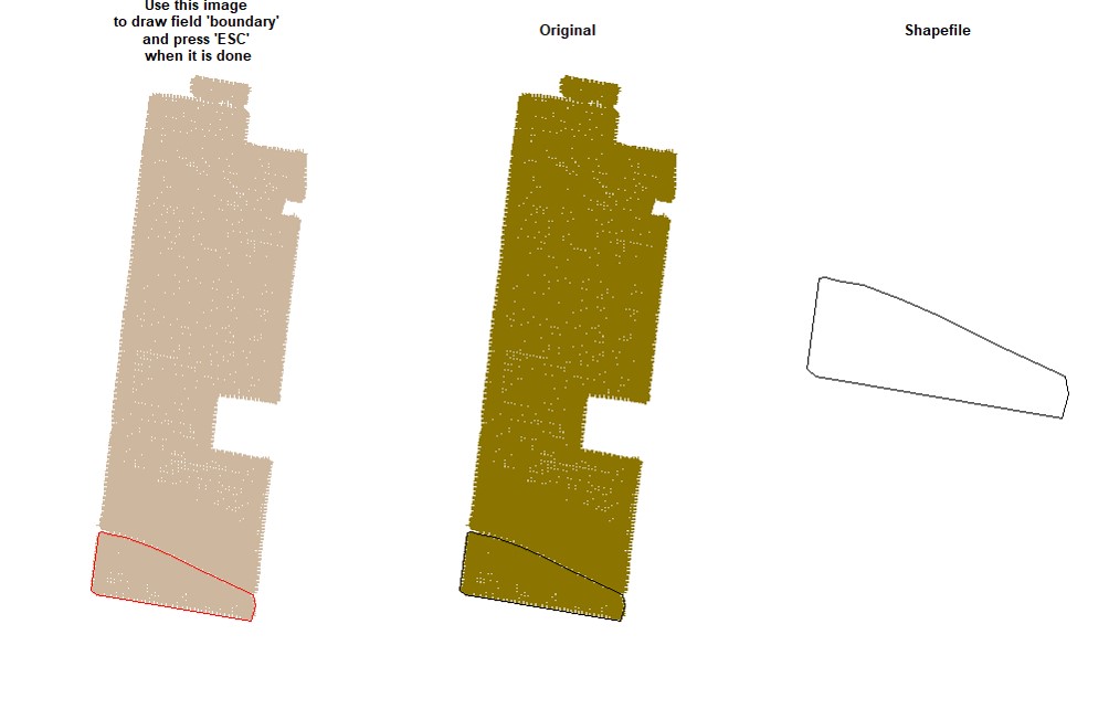
* **Drawing 3 different fields (Manually):** wzxhzdk:17

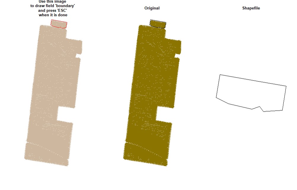
wzxhzdk:18

wzxhzdk:19

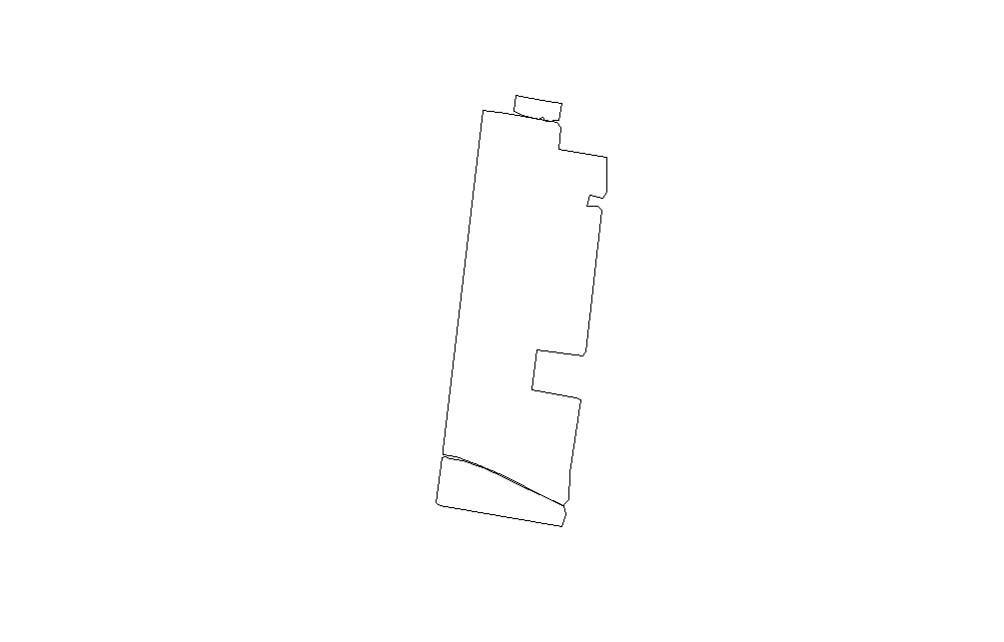
* **Combining fields on the same shapefile:** wzxhzdk:20

[Menu](#menu)

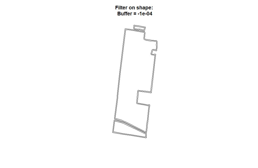
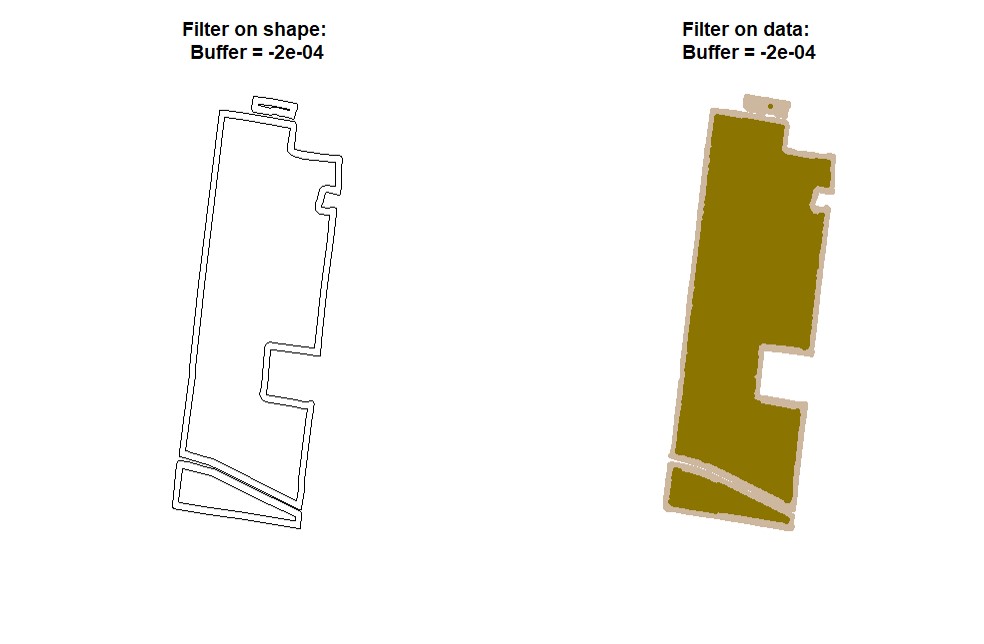
--------------------------------------------- #### 6. Buffering the field boundaries > Users can make a buffer around the field boundarys using a new shapefile (**Value must be negative**). Function **`bufferField`**. > Like in section 4, use either the provided code for unprojected data or projected data-- you will not need to run both sets of code. Under the cleanRfield update from March 2023, most input data sets will now be treated as projected data, even if they have the CRS WGS84. Be sure to check the 'LENGTHUNIT' atribute. * Only shapefile: wzxhzdk:21

* Making buffering and automatic filtering at the same time (Shapefile + Data). wzxhzdk:22

[Menu](#menu)

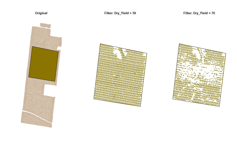
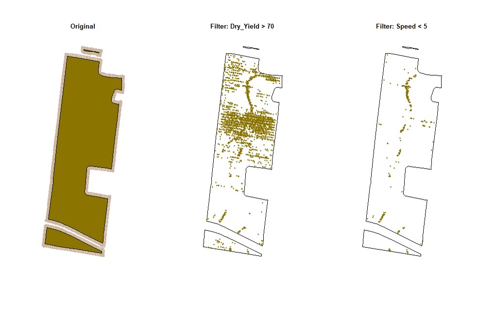
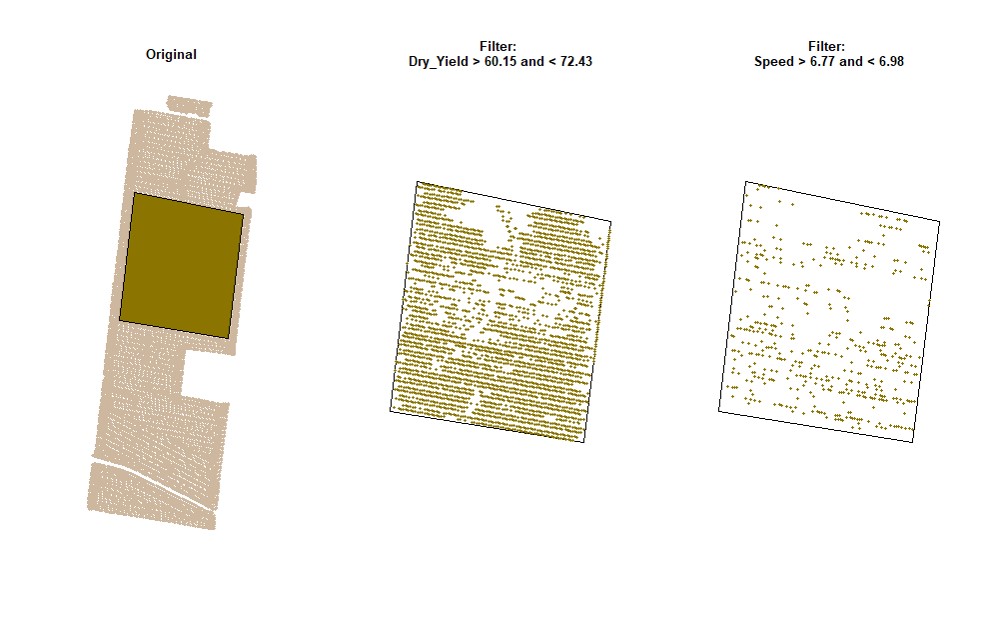
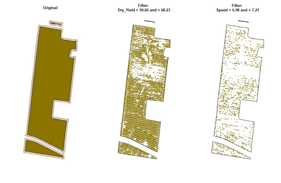
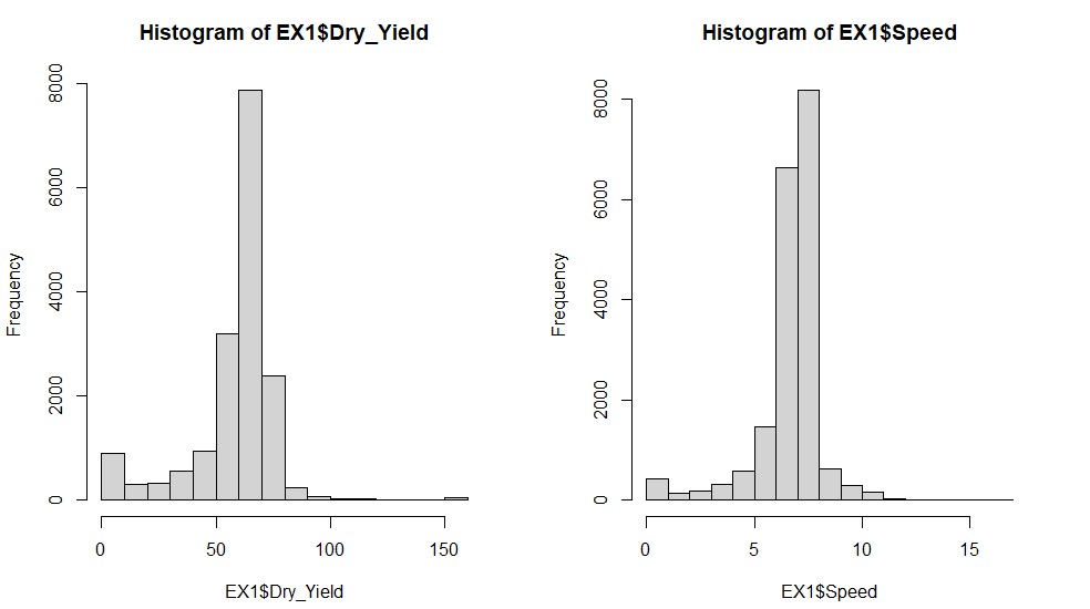
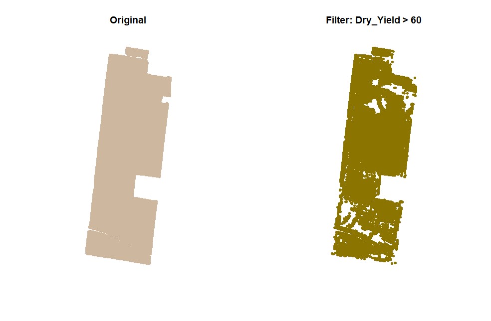
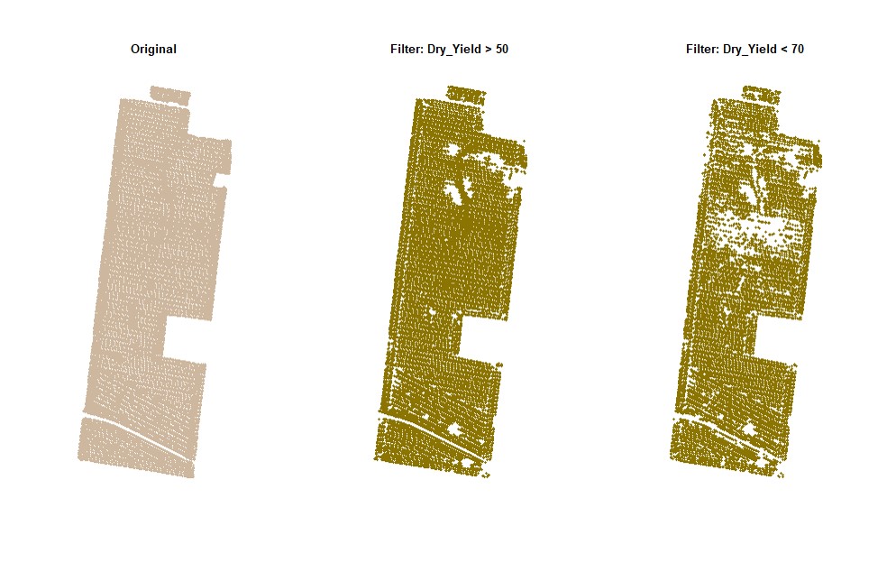
--------------------------------------------- #### 7. Filtering using data values > Users can filter spatial point data using values criteria. Function **`filterField`**. * Observing traits histograms: wzxhzdk:23

wzxhzdk:24

wzxhzdk:25

wzxhzdk:26

wzxhzdk:27

[Menu](#menu)

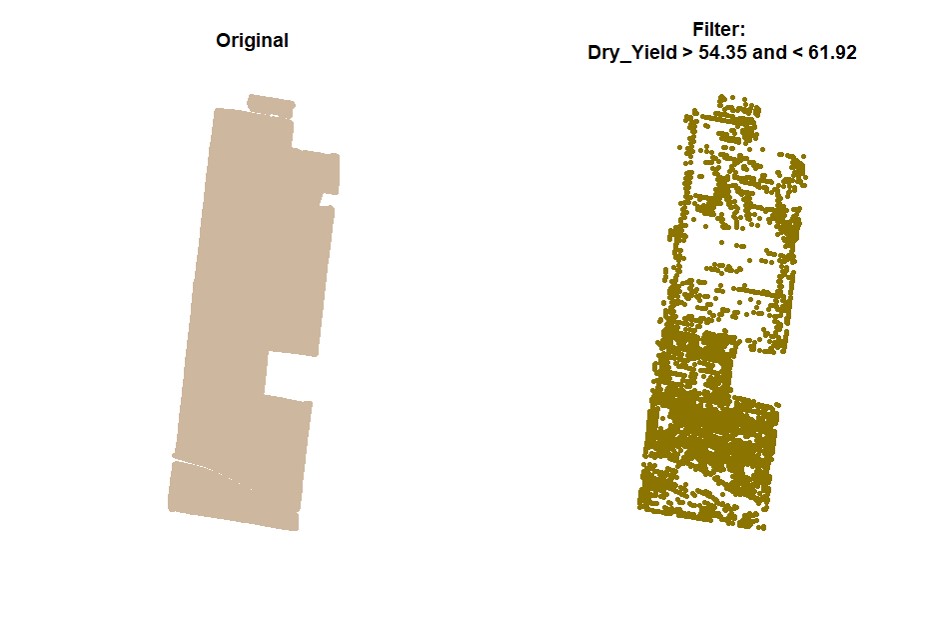
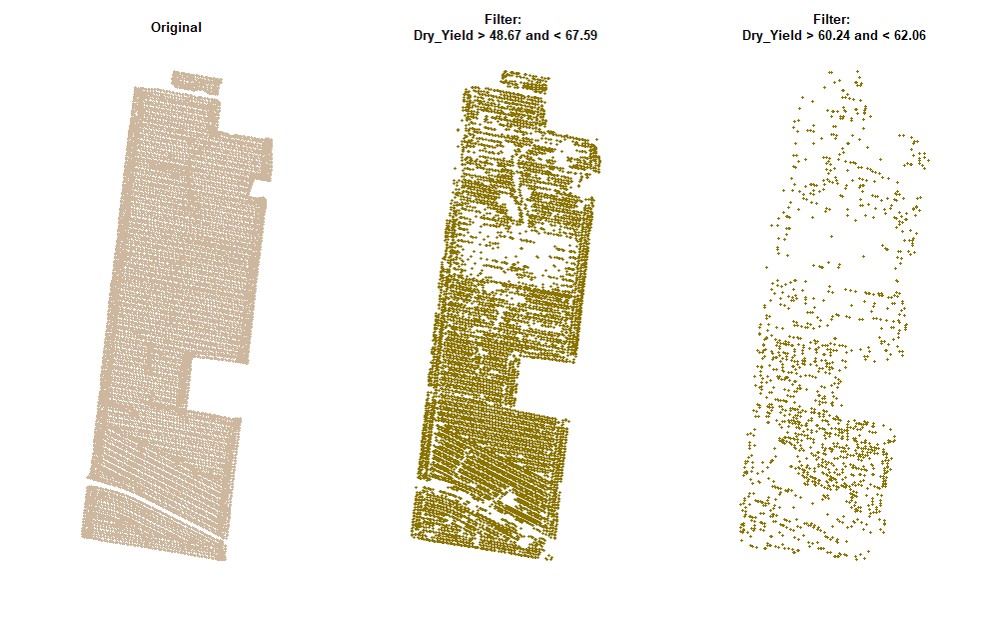
--------------------------------------------- #### 8. Filtering using standard deviation values > Filtering data can also be performed using standard deviation values for different traits. Function **`sdField`**. wzxhzdk:28

wzxhzdk:29

wzxhzdk:30

wzxhzdk:31

[Menu](#menu)

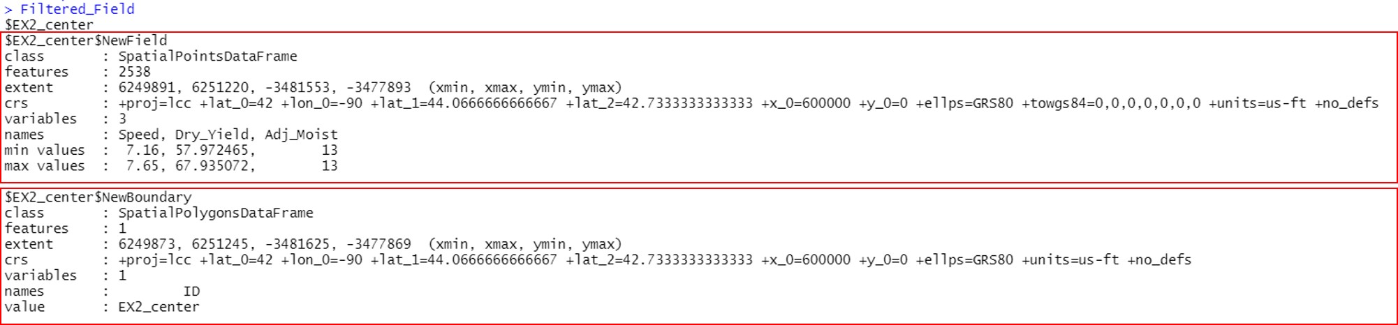
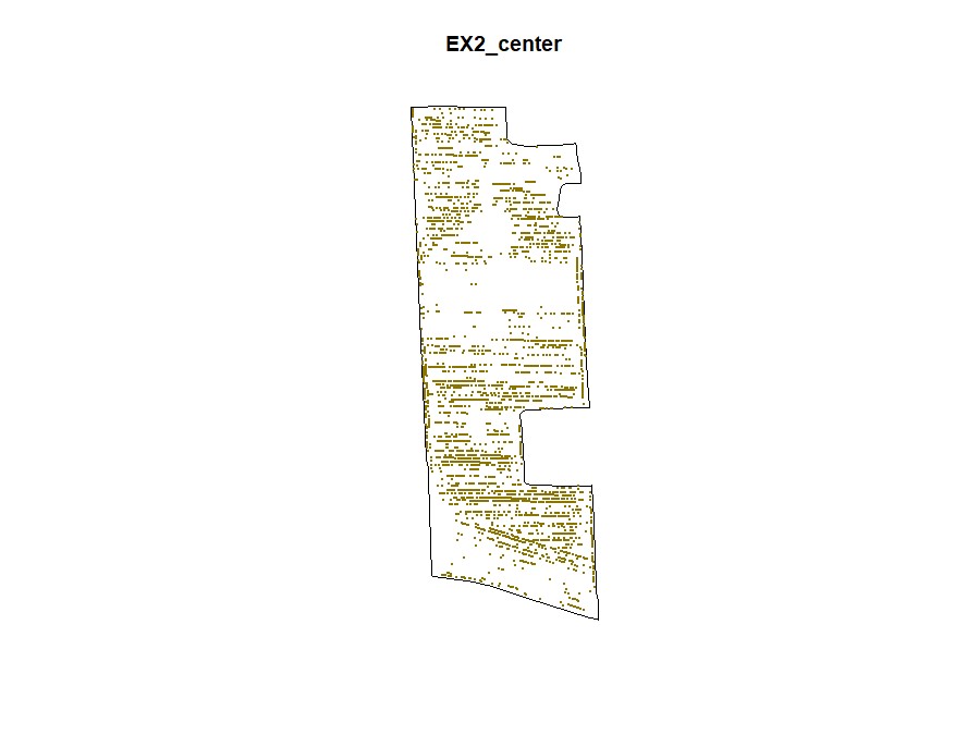
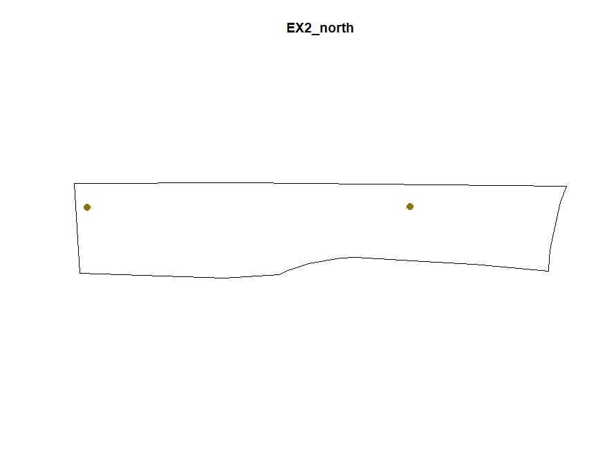
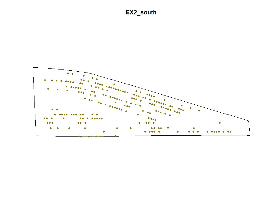
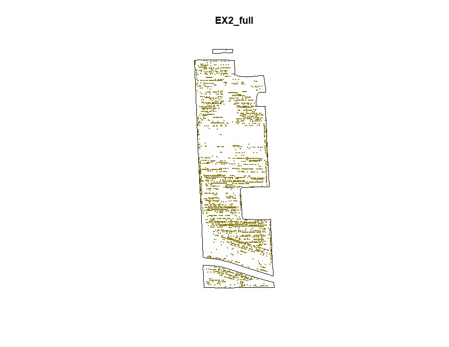
--------------------------------------------- #### 9. Evaluating multiple field on parallel > Download and unzip the projected data example below here [Parallel_Example.zip](https://drive.google.com/file/d/1-SywugJWDkbIrgalyUpe6wyRh0zRBGBN/view?usp=sharing). wzxhzdk:32

wzxhzdk:33

wzxhzdk:34

wzxhzdk:35

wzxhzdk:36

[Menu](#menu)

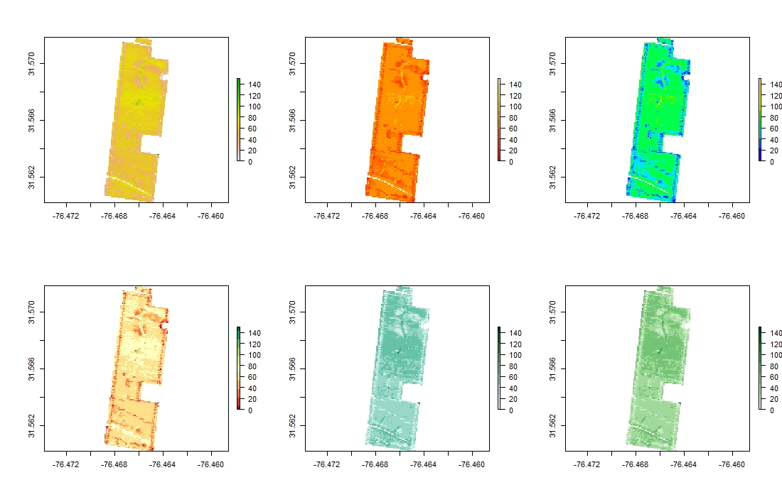
--------------------------------------------- #### 10. Making Maps * This example code uses the function `spplot()` from the **sp** package to visualze "SpatialPointsDataFrames" in the plot viewing pane in R studio. The demonstrated code is useful for visualizing data before or after filtering using **cleanRfield**. wzxhzdk:37

* If you prefer making visualizations using the package **ggplot2** , we recommend converting the data from "SpatialPointsDataFrames" to "sf" objects. wzxhzdk:38

[Menu](#menu)

--------------------------------------------- #### 11. Saving files * This example code uses the function `writeVector()` from the **terra** package to save "SpatVecor". wzxhzdk:39 [Menu](#menu)

--------------------------------------------- #### 12. Working with .csv and .txt files > If your data is stored as .csv or other file types, you can still utilizer cleanRfield by reading the data into a data frame in R before converting the data frame to a Spatial Points Data frame. This example uses a .csv file as the data source, but any data frame object in R that has coordinates can be converted to a spatial points data frame using this method regardless of data source file type. This data is in latitude and longitude (unprojected data). You will need to use a different CRS in the proj4string section if your data is projected. See the example code below and learn more about SpatialPoints in [the documentation for the package sp](https://cran.r-project.org/web/packages/sp/sp.pdf). Download the example: [EX3.csv](https://drive.google.com/file/d/1lIpsKyU-Xzcd0Hg-j7eo4J14NF4iy0wS/view?usp=sharing) wzxhzdk:40 [Menu](#menu)

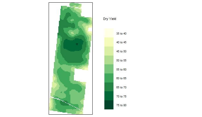
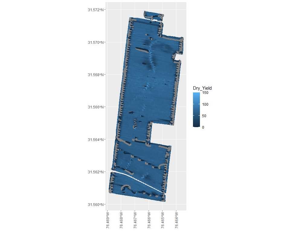
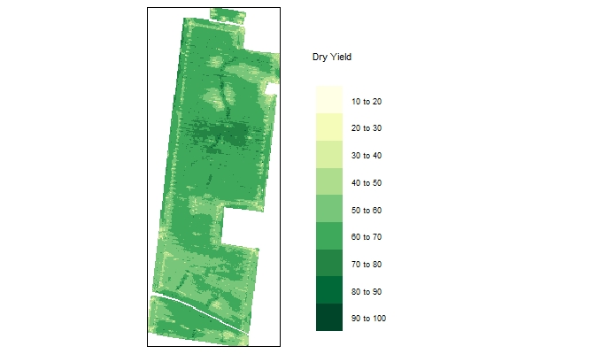
--------------------------------------------- #### 13. Interpolating yield maps > Users may want to interpolate their yield observations to create a raster data set for visualization or further data analysis. Below, we have provided some example code for interpolating yield maps using either inverse distance weighting (IDW) or ordinary kriging. In general, we recommend IDW due to its faster processing time for large data sets. > In this example code, we use the same example data (EX1) as in tutorial section 1. You may also need to install the package **tmap** before proceeding with the provided code. > The next code section provides an example for running IDW in R. Users will load the required pacakges, load and filter yield data, transform filtered data and the field boundary file, prepare an empty grid, run the IDW interpolation, and finally make a map to visualize the interpolation. Transformation is a step included in this workflow since the EX1 shapefile is not in a projected CRS, and transforming into a projected CRS helps align the yield map observations to the empty grid. Preparing the empty grid is necessary to determine the extent and resolution of the interpolation. wzxhzdk:41

> The following codes sections provides an example for interpolating via ordinary kriging in R. This workflow begins very similarly to the IDW interpolation workflow until we begin creating variogram models wzxhzdk:42

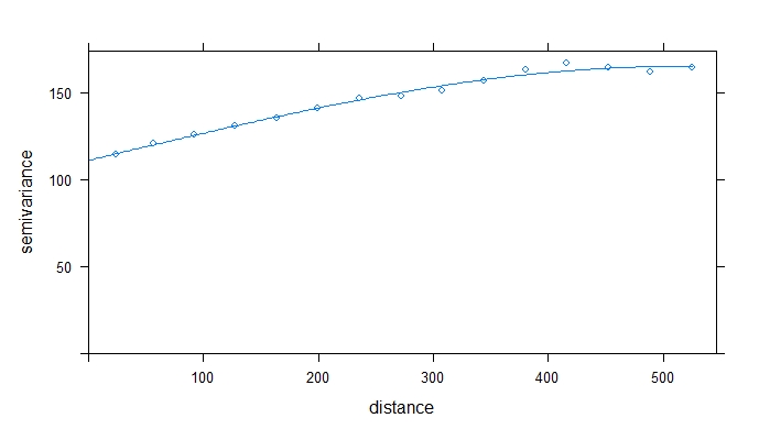
> The example variogram above had a range of ~509m, which indicates that yield observations that are <509m apart are spatially correlated. If you want to learn more about variograms, try [this blog post from GIS Geography](https://gisgeography.com/semi-variogram-nugget-range-sill/). Next, we will check that the data is not anisotrophic by developing 4 separate directional variograms. wzxhzdk:43

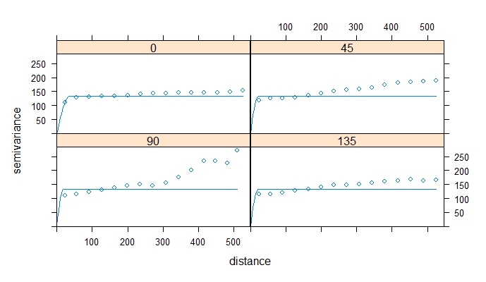
> There is not a commonly applied statistical test for anisotrophy, so this decision is a judgement call that each person will make a little differently. For distances <250m, these models are pretty similar. the data is not perfectly stationary, but in our judgement, it is not so anisotrophic that kriging would be inappropriate. If you perform directional variograms and there are very substantial differences between the models, we do not recommend kriging for interpolation. Instead, try another interpolation method that doesn't assume stationarity > Kriging takes a long time to compute, so in this example we will randomly sample 20% the yield observations before kriging to save time. Depending on your computer and your use for the kriged map, you may want to sample even fewer points, or krige using all observations. In this example we also used a lower resolution empty grid than in the IDW example to save computational time. wzxhzdk:44 > There's a reason most point-and-click softwares highly recommend not kriging yield maps. Even with just 20% of the observations, that took almost 5 min to run on my laptop. Running 50% of the observations takes me over 25 min. Fortunately, once the kriged surface is made, visualization is quick. wzxhzdk:45

> Regardless of interpolation method chosen, we highly recommend assessing the fit of your model using cross-validation and other methods. We do not provide code for assessing goodness of fit in this tutorial, but you can provide more information on this process from a variety of GIS tutorials. We find [Manuel Gimond's tutorial](https://mgimond.github.io/Spatial/interpolation-in-r.html) to be particularly helpful. [Menu](#menu)

--------------------------------------------- ### Forum for questions > This discussion group provides an online source of information about the cleanRfield package. Report a bug and ask a question at: * [https://groups.google.com/g/cleanRfield](https://groups.google.com/g/cleanRfield) ### Licenses > The R/cleanRfield package as a whole is distributed under [GPL-2 (GNU General Public License version 2)](https://www.gnu.org/licenses/gpl-2.0.en.html). ### Citation > coming soon... ### Author > * [Filipe Inacio Matias](https://github.com/filipematias23) > * [Emma Matcham](https://mobile.twitter.com/egmatcham) > * [Hunter Smith](https://www.linkedin.com/in/hunterdanielsmith/) ### Acknowledgments > * [Shawn Conley](https://coolbean.info/) > * [North Dakota State University](https://www.ndsu.edu/agriculture/academics/academic-units/plant-sciences) > * [University of Wisconsin - Madison](https://agronomy.wisc.edu/) [Menu](#menu)

filipematias23/cleanRfield documentation built on Aug. 6, 2023, 12:26 a.m.