README.md

In imadmali/stanode: R wrapper for modeling ODEs in Stan

rstanode

An ODE wrapper for RStan which takes a R function representation of an ODE system of equations and generates simulations via RStan. ~~There is also an option to fit data to the ODE system and estimate the initial conditions and/or the parameters.~~

Installation

To clone the repository and build the package locally run the following from R:

devtools::install_github("imadmali/stanode")

Example

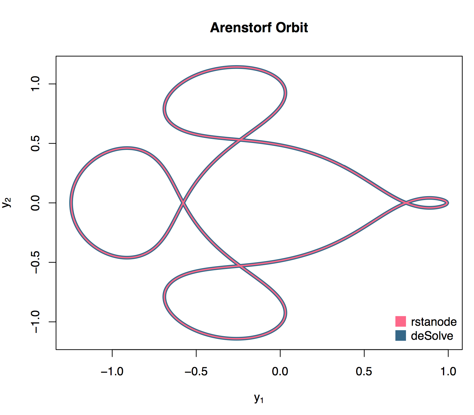
In this example we simulate an Arenstorf Orbit. For more examples see stan_ode.html

First define the ODE system as an R function (in this example we are using syntax that corresponds to the R package deSolve)

Arenstorf <- function(t, y, p) {
  with(as.list(c(y,p)), {
    D1 <- ((y[1] + mu1)^2 + y[2]^2)^(3/2)
    D2 <- ((y[1] - mu2)^2 + y[2]^2)^(3/2)
    dy1 <- y[3]
    dy2 <- y[4]
    dy3 <- y[1] + 2*y[4] - mu2*(y[1]+mu1)/D1 - mu1*(y[1]-mu2)/D2
    dy4 <- y[2] - 2*y[3] - mu2*y[2]/D1 - mu1*y[2]/D2
    return(list( c(dy1, dy2, dy3, dy4) ))
  })
}

Next specify the initial state values, parameter values, and time steps.

mu1 <- 0.012277471
pars <- c(mu1 = mu1, mu2 = 1 - mu1)
yini <- c(y1 = 0.994, y2 = 0,
          y3 = 0, y4 = -2.00158510637908252240537862224)
time_steps <- seq(from = 0, to = 18, by = 0.01)

Now we can simulate state values from the model at each time step with rstanode::stan_ode.

orbit_rstanode <- stan_ode(Arenstorf,
                           yini,
                           pars,
                           time_steps,
                           integrator = "rk45")
sims <- orbit_rstanode$simulations

To check we also simulate using deSolve::ode.

orbit_deSolve <- ode(func = Arenstorf, y = yini, parms = pars, times = time_steps)

Overlaying both results for state variable y1 and y2 we have the following plot.

plot(orbit_deSolve[,2], orbit_deSolve[,3], type = "l", col = "#336688", lwd = 5,
     main = "Arenstorf Orbit", xlab = expression(y[1]), ylab = expression(y[2]))
lines(sims[,2], sims[,3], col = "#FF6688", lwd = 2)
legend("bottomright", c("rstanode", "deSolve"), col = c("#FF6688","#336688"),
       pch = c(15,15), pt.cex = 2, bty = "n")

imadmali/stanode documentation built on May 3, 2019, 11:48 p.m.