In jackobailey/britpol: Data and Functions for Studying British Politics
# Load packages

library(britpol)
library(tidyverse)
library(lubridate)
library(here)


# Set knitr options

knitr::opts_chunk$set(
  collapse = TRUE,
  comment = "#>",
  fig.path = "man/figures/README-",
  out.width = "100%"
)
britpol

The {britpol} package makes analysing British political data quick and simple. It contains two pre-formatted datasets, plus a host of useful functions. The first dataset, pollbase, is a long-format version of Mark Pack's dataset of historic British public opinion polls combined with more recent data from Wikipedia. The second, pollbasepro, provides r format(nrow(pollbasepro), big.mark = ",") daily estimates of voting intention figures for each of Britain's three largest parties from r str_remove(format(min(pollbasepro$date), "%d %B %Y"), "^0") to r str_remove(format(max(pollbasepro$date), "%d %B %Y"), "^0").
To install the latest version of {britpol}, run the following code in R:
devtools::install_github("jackobailey/britpol")
Latest Polling Estimates from PollBasePro
# Get most recent pollbasepro estimates

txt_dta <-
  pollbasepro[pollbasepro$date == max(pollbasepro$date), ] %>%
  pivot_longer(
    cols = -date,
    names_to = c("party", ".value"),
    names_sep = "_"
    ) %>%
  arrange(desc(est)) %>%
  select(
    party,
    est,
    err
  ) %>%
  mutate(
    party =
      case_when(
        party == "con" ~ "Conservative Party",
        party == "lab" ~ "Labour Party",
        party == "lib" ~ "Liberal Democrats"
        ),
    lower = scales::percent(est - stats::qnorm(.975)*err, accuracy = 1),
    upper = scales::percent(est + stats::qnorm(.975)*err, accuracy = 1),
    share = scales::percent(est, accuracy = 1)
    )
# Define party colours

pty_cols <-
  c(
    "Conservative Party" = "#0087dc",
    "Labour Party" = "#d50000",
    "Liberals (Various Forms)" = "#fdbb30"
  )


# Create over time plot

timeplot <-
pollbasepro %>%
  pivot_longer(
    cols = -date,
    names_to = c("party", ".value"),
    names_sep = "_",
  ) %>%
  mutate(
    party =
      case_when(
        party == "con" ~ "Conservative Party",
        party == "lab" ~ "Labour Party",
        party == "lib" ~ "Liberals (Various Forms)"
      ) %>%
      factor(
        levels =
          c("Conservative Party",
            "Labour Party",
            "Liberals (Various Forms)"
          )
      )
  ) %>%
  ggplot(
    aes(
      x = date,
      y = est,
      ymin = est - qnorm(0.975)*err,
      ymax = est + qnorm(0.975)*err,
      colour = party,
      fill = party
    )
  ) +
  geom_ribbon(alpha = .3, colour = NA) +
  geom_line() +
  scale_colour_manual(values = pty_cols) +
  scale_fill_manual(values = pty_cols) +
  scale_y_continuous(
    breaks = seq(0, .6, by = .1),
    labels = scales::percent_format(accuracy = 1)
    ) +
  scale_x_date(
    breaks = seq.Date(as.Date("1955-01-01"), max(pollbasepro$date), by = "3 months"),
    labels = format(seq.Date(as.Date("1955-01-01"), max(pollbasepro$date), by = "3 months"), "%b %y")
    ) +
  coord_cartesian(
    ylim = c(0, 0.62),
    xlim = c(as_date("2019-12-12"), Sys.Date())
    ) +
  theme_minimal() +
    theme(
      legend.position = "none",
      legend.title = element_blank(),
      text = element_text(family = "Cabin", color = "black", size = 8),
      plot.title = element_blank(),
      plot.subtitle = element_text(family = "Cabin", size = rel(1), hjust = 0, margin = margin(b = 10)),
      axis.line = element_line(lineend = "round"),
      axis.title.x = element_blank(),
      axis.text.x = element_text(color = "black", size = rel(1)),
      axis.ticks.x = element_line(lineend = "round"),
      axis.title.y = element_text(family = "Cabin", face = "bold", size = rel(1)),
      axis.text.y = element_text(color = "black", size = rel(1)),
      strip.text = element_text(family = "Cabin", face = "bold", size = rel(1)),
      panel.spacing = unit(.3, "cm"),
      panel.grid.major.y = element_line(size = .5, lineend = "round"),
      panel.grid.minor.y = element_blank(),
      panel.grid.major.x = element_blank(),
      panel.grid.minor.x = element_blank()
    ) +
  labs(
    title = paste0("British Poll of Polls, ", str_remove(format(max(pollbasepro$date), "%d %B %Y"), "^0")),
    colour = "Party",
    fill = "Party",
    y = "Vote Share",
    caption = "Made using PollBasePro by @PoliSciJack, @markpack, and @mansillo"
  )


# Output plot

ggsave(
  filename = "timeplot_gh.png",
  plot = timeplot,
  path = here("documentation", "_assets"),
  width = 3.5,
  height = 2.3,
  units = "in",
  dpi = 320,
  bg = "white"
)
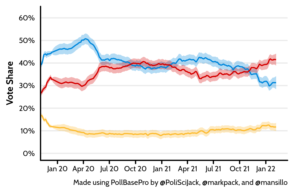
British Poll of Polls, r str_remove(format(max(pollbasepro$date), "%d %B %Y"), "^0"):
r txt_dta$party[1]: r paste0(txt_dta$share[1], " (", txt_dta$lower[1], " to ", txt_dta$upper[1], ")")r txt_dta$party[2]: r paste0(txt_dta$share[2], " (", txt_dta$lower[2], " to ", txt_dta$upper[2], ")")r txt_dta$party[3]: r paste0(txt_dta$share[3], " (", txt_dta$lower[3], " to ", txt_dta$upper[3], ")")
pollbasepro suggests that the r txt_dta$party[1] r ifelse(txt_dta$party[1] %in% c("Conservative Party", "Labour Party"), "is", "are") the largest party in Britain. They hold a lead over the r txt_dta$party[2] of around r paste0(scales::percent(txt_dta$est[1] - txt_dta$est[2], suffix = "pp"), " (", scales::percent((txt_dta$est[1] - txt_dta$est[2]) - qnorm(.975)*sqrt(txt_dta$err[1]^2 + txt_dta$err[2]^2), suffix = "pp"), " to ", scales::percent((txt_dta$est[1] - txt_dta$est[2]) + qnorm(.975)*sqrt(txt_dta$err[1]^2 + txt_dta$err[2]^2), suffix = "pp"), ")"). This puts the r txt_dta$party[2] in second and the r txt_dta$party[3] in third.
Notes, Usage, and Attribution
{britpol}, pollbase, and pollbasepro will change over time as elections come and go. Users should use only the most recent version of the package when conducting their analyses. Like any project, some minor mistakes might have crept into the code. If you think that you have found an error or would like to make a recommendation for a future update, please raise an issue.
You may also use the {britpol} codebase for your own purposes in line with its license. But you must do so with attribution. That is, you may reproduce, reuse, and adapt the code as you see fit, but must state in each case that you used {britpol} to produce your work. The relevant citations are as follows:
britpol
- Documentation: Bailey, J. (
r format(Sys.Date(), format = "%Y")) britpol vr packageVersion("britpol"): User Guide and Data Codebook. Retrieved from https://doi.org/10.17605/OSF.IO/2M9GB.
PollBasePro
-
Data: Bailey, J., M. Pack, and L. Mansillo (r format(Sys.Date(), format = "%Y")) PollBasePro: Daily Estimates of Aggregate Voting Intention in Great Britain from r format(min(pollbasepro$date), "%Y") to r format(max(pollbasepro$date), "%Y") v.r packageVersion("britpol") [computer file], r format(Sys.Date(), format = "%B %Y"). Retrieved from https://doi.org/10.7910/DVN/3POIQW.
-
Paper: Bailey, J., M. Pack, and L. Mansillo (r format(Sys.Date(), format = "%Y")) PollBasePro: Daily Estimates of Aggregate Voting Intention in Great Britain from r format(min(pollbasepro$date), "%Y") to r format(max(pollbasepro$date), "%Y"). Retrieved from doi.
jackobailey/britpol documentation built on Aug. 6, 2023, 2:30 a.m.
R Package Documentation
Browse R Packages
We want your feedback!
Note that we can't provide technical support on individual packages. You should contact the package authors for that.
# Load packages library(britpol) library(tidyverse) library(lubridate) library(here) # Set knitr options knitr::opts_chunk$set( collapse = TRUE, comment = "#>", fig.path = "man/figures/README-", out.width = "100%" )
britpol
The {britpol} package makes analysing British political data quick and simple. It contains two pre-formatted datasets, plus a host of useful functions. The first dataset, pollbase, is a long-format version of Mark Pack's dataset of historic British public opinion polls combined with more recent data from Wikipedia. The second, pollbasepro, provides r format(nrow(pollbasepro), big.mark = ",") daily estimates of voting intention figures for each of Britain's three largest parties from r str_remove(format(min(pollbasepro$date), "%d %B %Y"), "^0") to r str_remove(format(max(pollbasepro$date), "%d %B %Y"), "^0").
To install the latest version of {britpol}, run the following code in R:
devtools::install_github("jackobailey/britpol")
Latest Polling Estimates from PollBasePro
# Get most recent pollbasepro estimates txt_dta <- pollbasepro[pollbasepro$date == max(pollbasepro$date), ] %>% pivot_longer( cols = -date, names_to = c("party", ".value"), names_sep = "_" ) %>% arrange(desc(est)) %>% select( party, est, err ) %>% mutate( party = case_when( party == "con" ~ "Conservative Party", party == "lab" ~ "Labour Party", party == "lib" ~ "Liberal Democrats" ), lower = scales::percent(est - stats::qnorm(.975)*err, accuracy = 1), upper = scales::percent(est + stats::qnorm(.975)*err, accuracy = 1), share = scales::percent(est, accuracy = 1) )
# Define party colours pty_cols <- c( "Conservative Party" = "#0087dc", "Labour Party" = "#d50000", "Liberals (Various Forms)" = "#fdbb30" ) # Create over time plot timeplot <- pollbasepro %>% pivot_longer( cols = -date, names_to = c("party", ".value"), names_sep = "_", ) %>% mutate( party = case_when( party == "con" ~ "Conservative Party", party == "lab" ~ "Labour Party", party == "lib" ~ "Liberals (Various Forms)" ) %>% factor( levels = c("Conservative Party", "Labour Party", "Liberals (Various Forms)" ) ) ) %>% ggplot( aes( x = date, y = est, ymin = est - qnorm(0.975)*err, ymax = est + qnorm(0.975)*err, colour = party, fill = party ) ) + geom_ribbon(alpha = .3, colour = NA) + geom_line() + scale_colour_manual(values = pty_cols) + scale_fill_manual(values = pty_cols) + scale_y_continuous( breaks = seq(0, .6, by = .1), labels = scales::percent_format(accuracy = 1) ) + scale_x_date( breaks = seq.Date(as.Date("1955-01-01"), max(pollbasepro$date), by = "3 months"), labels = format(seq.Date(as.Date("1955-01-01"), max(pollbasepro$date), by = "3 months"), "%b %y") ) + coord_cartesian( ylim = c(0, 0.62), xlim = c(as_date("2019-12-12"), Sys.Date()) ) + theme_minimal() + theme( legend.position = "none", legend.title = element_blank(), text = element_text(family = "Cabin", color = "black", size = 8), plot.title = element_blank(), plot.subtitle = element_text(family = "Cabin", size = rel(1), hjust = 0, margin = margin(b = 10)), axis.line = element_line(lineend = "round"), axis.title.x = element_blank(), axis.text.x = element_text(color = "black", size = rel(1)), axis.ticks.x = element_line(lineend = "round"), axis.title.y = element_text(family = "Cabin", face = "bold", size = rel(1)), axis.text.y = element_text(color = "black", size = rel(1)), strip.text = element_text(family = "Cabin", face = "bold", size = rel(1)), panel.spacing = unit(.3, "cm"), panel.grid.major.y = element_line(size = .5, lineend = "round"), panel.grid.minor.y = element_blank(), panel.grid.major.x = element_blank(), panel.grid.minor.x = element_blank() ) + labs( title = paste0("British Poll of Polls, ", str_remove(format(max(pollbasepro$date), "%d %B %Y"), "^0")), colour = "Party", fill = "Party", y = "Vote Share", caption = "Made using PollBasePro by @PoliSciJack, @markpack, and @mansillo" ) # Output plot ggsave( filename = "timeplot_gh.png", plot = timeplot, path = here("documentation", "_assets"), width = 3.5, height = 2.3, units = "in", dpi = 320, bg = "white" )
British Poll of Polls, r str_remove(format(max(pollbasepro$date), "%d %B %Y"), "^0"):
r txt_dta$party[1]:r paste0(txt_dta$share[1], " (", txt_dta$lower[1], " to ", txt_dta$upper[1], ")")r txt_dta$party[2]:r paste0(txt_dta$share[2], " (", txt_dta$lower[2], " to ", txt_dta$upper[2], ")")r txt_dta$party[3]:r paste0(txt_dta$share[3], " (", txt_dta$lower[3], " to ", txt_dta$upper[3], ")")
pollbasepro suggests that the r txt_dta$party[1] r ifelse(txt_dta$party[1] %in% c("Conservative Party", "Labour Party"), "is", "are") the largest party in Britain. They hold a lead over the r txt_dta$party[2] of around r paste0(scales::percent(txt_dta$est[1] - txt_dta$est[2], suffix = "pp"), " (", scales::percent((txt_dta$est[1] - txt_dta$est[2]) - qnorm(.975)*sqrt(txt_dta$err[1]^2 + txt_dta$err[2]^2), suffix = "pp"), " to ", scales::percent((txt_dta$est[1] - txt_dta$est[2]) + qnorm(.975)*sqrt(txt_dta$err[1]^2 + txt_dta$err[2]^2), suffix = "pp"), ")"). This puts the r txt_dta$party[2] in second and the r txt_dta$party[3] in third.
Notes, Usage, and Attribution
{britpol}, pollbase, and pollbasepro will change over time as elections come and go. Users should use only the most recent version of the package when conducting their analyses. Like any project, some minor mistakes might have crept into the code. If you think that you have found an error or would like to make a recommendation for a future update, please raise an issue.
You may also use the {britpol} codebase for your own purposes in line with its license. But you must do so with attribution. That is, you may reproduce, reuse, and adapt the code as you see fit, but must state in each case that you used {britpol} to produce your work. The relevant citations are as follows:
britpol
- Documentation: Bailey, J. (
r format(Sys.Date(), format = "%Y")) britpol vr packageVersion("britpol"): User Guide and Data Codebook. Retrieved from https://doi.org/10.17605/OSF.IO/2M9GB.
PollBasePro
-
Data: Bailey, J., M. Pack, and L. Mansillo (
r format(Sys.Date(), format = "%Y")) PollBasePro: Daily Estimates of Aggregate Voting Intention in Great Britain fromr format(min(pollbasepro$date), "%Y")tor format(max(pollbasepro$date), "%Y")v.r packageVersion("britpol")[computer file],r format(Sys.Date(), format = "%B %Y"). Retrieved from https://doi.org/10.7910/DVN/3POIQW. -
Paper: Bailey, J., M. Pack, and L. Mansillo (
r format(Sys.Date(), format = "%Y")) PollBasePro: Daily Estimates of Aggregate Voting Intention in Great Britain fromr format(min(pollbasepro$date), "%Y")tor format(max(pollbasepro$date), "%Y"). Retrieved from doi.
R Package Documentation
Browse R Packages
We want your feedback!
Note that we can't provide technical support on individual packages. You should contact the package authors for that.
Embedding an R snippet on your website
Add the following code to your website.
For more information on customizing the embed code, read Embedding Snippets.