README.md

In jakobbossek/grapherator: A Modular Multi-Step Graph Generator

grapherator: Modular graph generation

Introduction

Due to lack of real world data comparisson of algorithms for graph problems is most often carried out on artificially generated graphs. The R package grapherator implements a modular approach to benchmark graph generation focusing on undirected, weighted graphs. The graph generation process follows a three-step procedure:

1. Node generation,
2. edge generation and finally
3. edge weight generation.

Each step may be repeated multiple times with different generators before the transition to the next step is conducted.

Example

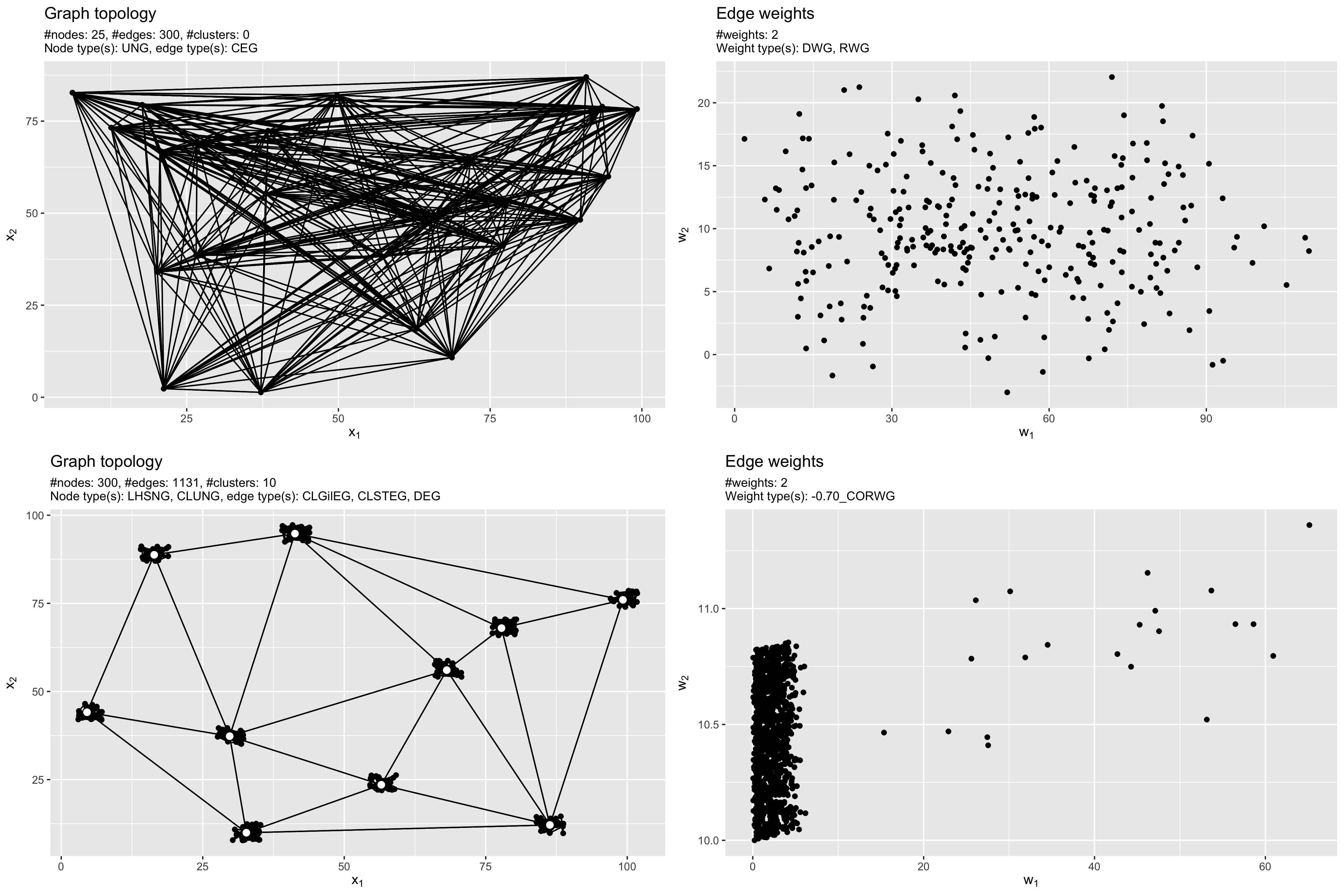
Here, we first generate a bi-criteria complete graph with n = 25 nodes and each two conflicting weights per edge. The first weight is the Euclidean distance of node coordinates in the Euclidean plane [0, 10] x [0, 10]. The second objective follows a N(5, 1.5)-distribution, i.e., a normal distribution with mean 5 and standard deviation 1.5.

set.seed(1)
g1 = graph(lower = 0, upper = 10)
g1 = addNodes(g1, n = 25, generator = addNodesUniform)
g1 = addWeights(g1, generator = addWeightsDistance, method = "euclidean")
g1 = addWeights(g1, generator = addWeightsRandom, method = rnorm, mean = 5, sd = 1.5)
print(g1)
do.call(gridExtra::grid.arrange, plot(g1))

The next example demonstrates multiple iterations of each step to create a complex, clustered, connected network with different edge generators applied for establishing links within clusters and between cluster centers respectively. Detailed description: First, 10 cluster centers are placed via Latin-Hypercube-Sampling (LHS). Next, each cluster is crowded with 29 additional nodes by uniform sampling around the cluster center. Edge generation is done by randomly adding an edge between each two nodes in a cluster with small probability p = 0.2. To ensure connectivity, the spanning tree edge generator is applied. The last step of edge generation connects the clusters via Delauney triangulation. In a final step, two negatively correlated weights are added.

set.seed(1)
g2 = graph(lower = 0, upper = 100)
g2 = addNodes(g2, n = 10, generator = addNodesLHS)
g2 = addNodes(g2, n = 29, by.centers = TRUE, generator = addNodesUniform, lower = c(0, 0), upper = c(5, 5))
g2 = addEdges(g2, type = "intracluster", generator = addEdgesGilbert, p = 0.2)
g2 = addEdges(g2, type = "intracluster", generator = addEdgesSpanningTree)
g2 = addEdges(g2, type = "intercenter", generator = addEdgesDelauney)
g2 = addWeights(g2, generator = addWeightsCorrelated, rho = -0.7)
print(g2)
do.call(gridExtra::grid.arrange, plot(g2))

The following image shows both example graphs g1 and g2. The topology is shown in the left column, while a scatterplot of the weights is visualized in the right column.

See the package vignettes for more examples and thorough description.

Installation Instructions

Install the CRAN release version via:

install.packages("grapherator")

If you are interested in trying out and playing around with the current development version use the devtools package and install directly from GitHub:

install.packages("devtools", dependencies = TRUE)
devtools::install_github("jakobbossek/grapherator")

Contributing to grapherator

If you encounter problems using this software, e.g., bugs or insufficient/misleading documentation, or you simply have a question, feel free to open an issue in the issue tracker. In order to reproduce potential problems, please provide a minimal and reproducible code example.

Contributions to this software package are welcome via pull requests and will be merged at the sole discretion of the author.

Related work

The following R packages provide some methods to generate random graphs:

• igraph: Network Analysis and Visualization Includes some methods to generate classical Erdos-Renyi random graphs as well as more recent models, e.g., small-world graphs.
• netgen: Network Generator for Combinatorial Graph Problems Contains some methods to generate complete graphs especially for benchmarking Travelling-Salesperson-Problem solvers.
• bnlearn: Bayesian Network Structure Learning, Parameter Learning and Inference Function bnlearn::random.graph implements some algorithms to create graphs.

More interesting libraries:

• Graphcuisine Provides an interactive Evolutionary Algorithm to create random graphs with certain user-guided characteristics or maximal similarity to a given baseline graph.
• NetworkX Powerful python package which provides many methods to generate classic and random networks.

jakobbossek/grapherator documentation built on Oct. 4, 2021, 11:03 a.m.