In jonathan-mcmillan/csci3500: immune Cell Analysis Tool

iCAT aims to (1) identify TCR sequences that are significantly associated with target samples and (2) to binary-classify unkown samples. Users can either perform analysis using the Shiny graphical user interface, or directly on an R interpreter.

Graphical User Interface Workflow

In R:

library(iCAT)
iCATinteractive()

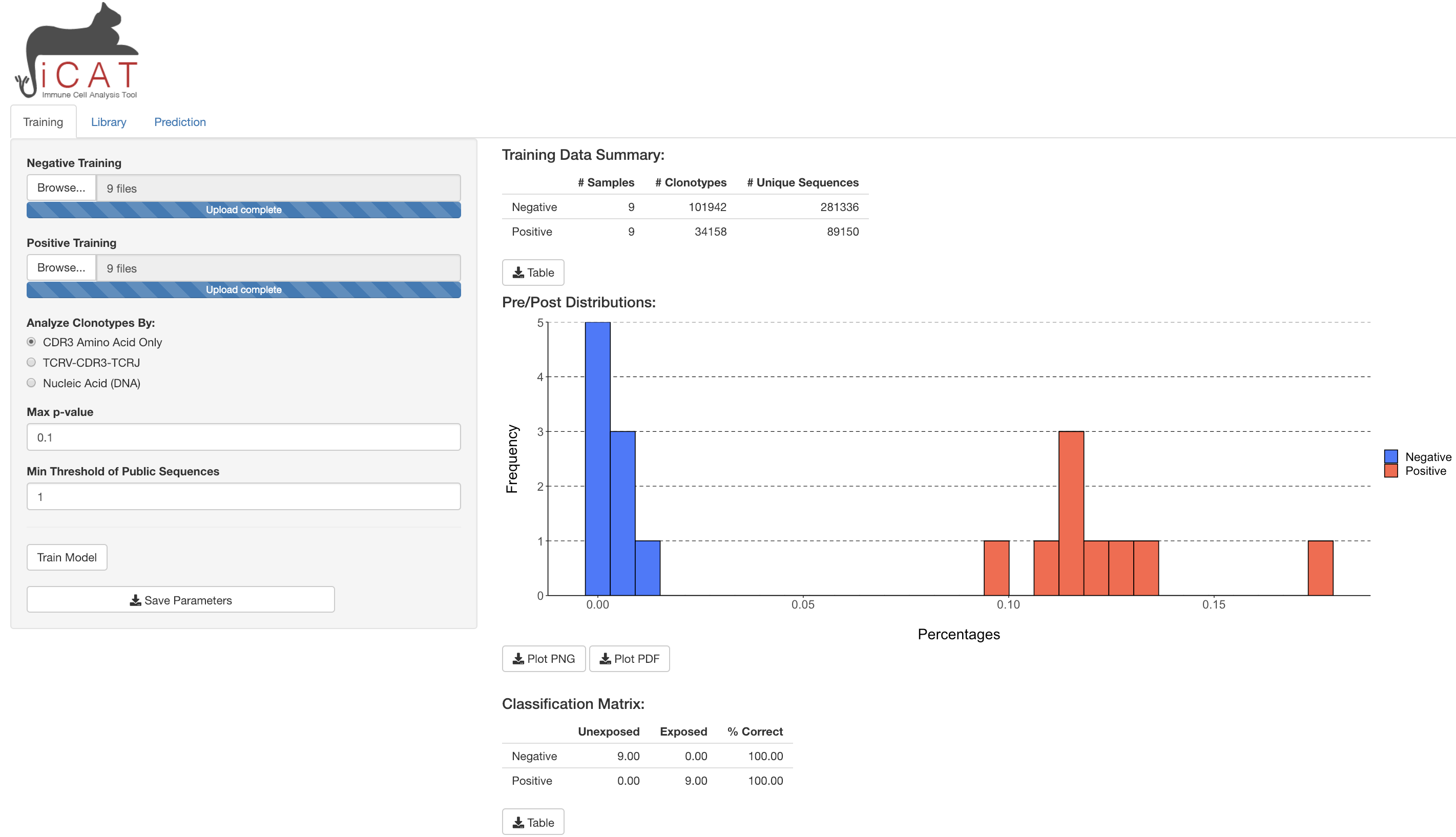
This will launch a graphical user interface (GUI) for iCAT. The GUI has three tabs, separating major functionalities: training, library, and prediction.

Training:

knitr::opts_chunk$set(collapse = TRUE, out.width="100%")

1) In the Training tab, enter your negative training samples (naïve, unexposed, uninfected, pre-infection, etc) using the Browse button.

Individual samples’ sequencing data should be in .tsv format.

2) Repeat step 1 for positive training samples (exposed, infected, etc.)

3) Choose if you want to analyze data by: - CDR3 Amino Acid Sequence (TCRs will need the same CDR3 region to be called ‘Identical’) - TCRV-CDR3-TCRJ (TCRs will need the same TCRBV segment, CDR3 region, and TCRJ segment to be called ‘Identical’) Recommended - Nucleic Acid (DNA) (TCRs will need the exact same DNA rearrangements/sequence across TCRBV, CDR3, and TCRJ)

4) Choose the Max p-value, which determines the minimal degree of statistical significance that iCAT will accept as being potentially "associated" with the positive group. Defaults to p < 0.1.

5) Choose the Min Threshold of Public Sequences, which determines the minimum number of training samples a TCR sequence must be observed in to be considered as potentially "associated" with the positive group. Defaults to 1. Recommend setting at 10% of positive training samples. E.g. if there are 30 positive training samples, a recommended minimum threshold is 3.

6) Once all options are selected click Train Model

A progress bar will show on the bottom-right corner to update on the satatus of training. After finishing, the training tab will show some exploratory tables and a figure regarding the training data and the model built, which can all be downloaded to the user's machine. In addition, the library and prediction tab will unlock.

Library:

The Library tab displays a table consisting of the "target associated receptor sequences" (TARS), determined to be statistically associated with exposure to the target/agent/pathogen. The table displays each sequence, number of positive and negative training samples the sequence is present in/absent from, and how statistically associated the sequence is to the positive training data (p-value). The table can be downloaded to the user's computer for further analysis using excel, commandline, etc using the download Table button below the table.

Prediction:

The Prediction tab allows the user to add sequencing data from unknown samples (e.g. not included in the previous training data) for classification as "Positive" or "Negative" and determining the accuracy of the diagnostic assay.

1) Use the Browse button to add samples for prediction. Multiple samples may be uploaded simultaneously. 2) Click Predict Independent Sample.

A table will appear after analysis is complete. The table displays sample names along with the prediction "Positive" (red)/ "Negative" (blue), and displays the ‘%TARS’: the percent of individual sequences from the sample that are included in the TARS library. The prediction results can be downloaded as a table.

R-interface Workflow

After loading iCAT with library(iCAT)

1) Define the parameters you would like to use for building the model:

FIELD <- "vGeneName aminoAcid jGeneName"
P_CUTOFF <- 0.1
MIN_PUBLIC <- 2

2) Make lists of .tsv Positive and Negative training samples:

listPos <- tsvDir("path/to/positve/samples/")
listNeg <- tsvDir("path/to/negative/samples/")

• optional Collect summary statistics about training samples:

trnStats(listPos, listNeg, FIELD)
#>         # Samples # Clonotypes # Unique Sequences
#>Negative         9       101942             281336
#>Positive         9        34158              89150

3) Read in Positive and Negative training samples:

naive <- readTrn(listNeg, FIELD, "naive")
vaccs <- readTrn(listPos, FIELD, "vacc")       

4) Build a model using the training data:

mod <- train(naive, vaccs, listNeg, listPos, FIELD, P_CUTOFF, MIN_PUBLIC, NULL)

• optional Produce a table estimating the classification accuracy of the model:

classMat(mod)

• optional Produce a figure showing % of TCR associated with positve samples in positive and negative samples:

plotHist(mod)

• optional Produce the library of TCR sequences associated with positve samples:

getLib(mod) 

jonathan-mcmillan/csci3500 documentation built on Jan. 31, 2020, 12:25 a.m.