README.md

In khufkens/cropmonitor: IFPRI cellphone based crop monitoring application

Cropmonitor

The IFPRI crop monitor R package calculates greenness indices (Gcc and GRVI) for cellphone based data acquisitions within the context of cellphone based index-based micro-insurance.

The tool allows for the visualization of the database, but requires a local database to be updated (see below).

Installation

Install the cropmonitor R package using the following code:

if (!require(devtools)) install.packages("devtools")
install_github("khufkens/cropmonitor")
library(cropmonitor)

Use

Data is generated based upon a database dump provided as a .dta file (this format can, and should be changed for transparency reasons).

If no local database exists the local database is generated and populated. The local database is called cropmonitor.json and by default located in the your home directory in an automatically generated data folder called /users/testuser/cropmonitor. If the cropmonitor.json file exits, it is compared with the provided .dta file and updated if necessary.

In addition, the raw image data will be downloaded from the IFPRI servers onto your workstation. The raw data is stored in a subfolder in the data folder. This folder is called images and matching thumbnails are stored in a thumbs folder. A final output folder is also created to hold the output of plotting functions. This folder will not be generated until the plotting function is called for the first time. The file structure is outlined in the graph below. A different path for data storage can be specified, but is not recommended.

/users/testuser/cropmonitor
    │   cropmonitor.json
    └─── images
    │   └───user_id
    │       │───cropsite_id
    │       │   ...
    |
    └─── thumbs
    |   └───user_id
    |       │───cropsite_id
    |       │   ...
    |
    └─── output
            figure.pdf
             ...

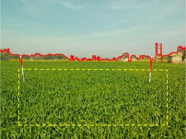
The thumbnails have annotations on them pertaining to the automatically selected region of interest (ROI, yellow dashed line) and the horizon line (red full line) which assists in this process.

# How to update the local database
batch.process.database(database = "Pictures Data CLEAN 03_03_17.dta")

Once the database is generated operations on the data are quickly plotted using the following function call.

# Plotting the data without additional information
plot.sites(database = "~/cropmonitor/cropmonitor.json")

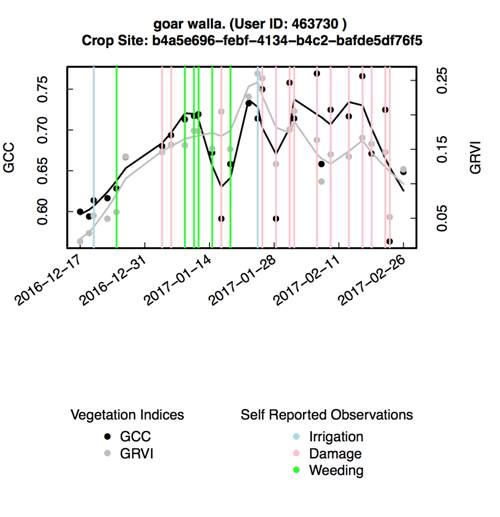
In addition to plotting data as simple time series, one can include field surveys as collected together with the image acquisitions in the field. If an XLSX file is provided, this data will be merged and visualized.

# Plotting the data with additional 'questionaire' information
plot.sites(database = "~/cropmonitor/cropmonitor.json",
             questionaire = "~/cropmonitor/questionaire.xlsx)

An example plot is shown below.

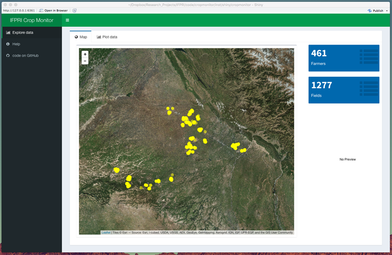
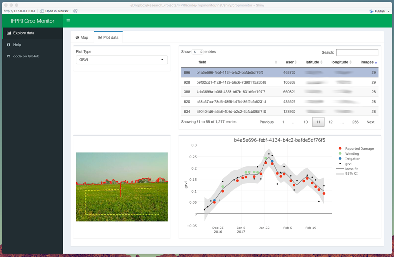
Finally to access the interactive graphical user interface for exploring the data execute the following command.

# Start the graphical user interface, to explore the data
cropmonitor()

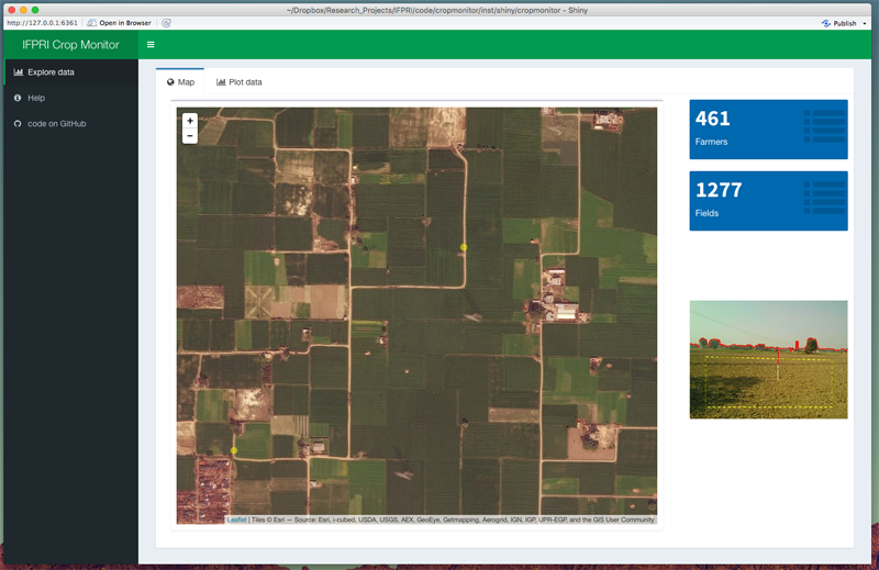
The opening screens shows the site locations as yellow dots on the map. Clicking on the dots will show you a preview at the location (a cellphone image).

On the second window one can scroll through all data (time series plotted by field). The displayed table can be sorted based on, farmer name, field name, latitude, longitude or number of images collected. The time series plotted can be changed using the dropdown box on the left hand side.

Clicking on a site location in the table will bring up a graph (bottom right) and a preview of the field site (bottom left). In addition to the normal time series a fitted curve is shown together with it's 95% confidence intervals, as well as details regarding management such as weeding, irrigation and self-reported damage.

khufkens/cropmonitor documentation built on May 31, 2019, 8:29 a.m.