README.md

In kmayerb/spcv: a minimalist package for anticipating prediction errors in spatial interpolation through cross validation

spcv

a minimalist R package for anticipating prediction errors in spatial interpolation through cross validation

In Search of a Goldilocks Interpolator

Code for plots in this README.md can be found as a RMarkdown document in the /proto-vignettes/ folder

What is spcv?

spcv, short for spatial cross validation, is a minimalist R package for anticipating prediction errors in spatially interpolated data. For now, it’s based on hold one out cross validation, and it is meant to work with the R spatial statistics package gstat.

spcv can currently be used to examine the magnitude and distribution of errors generated by inverse distance weighted (IDW) interpolations. With minor modification it could be adapted to cross validate other gstat interpolators (i.e. simple, ordinary, block, and universal kriging).

What is inverse distance weighting?

Inverse distance weighting (or IDW for short) is a simple, but flexible, interpolation method. An estimate at an unknown point is calculated from a weighted average of the values available at the known points, where the weights assigned to each point is an inverse function of distance ( usually 1 / dist(x[i]-x[j] )^p ) to the interpolation location. The power parameter (p) can be increased to lend greater weight to near-field points.

IDW differs from kriging interpolation in that it does not rely on distributional assumptions about the underlying data. IDW is easy to tune and implement, but it offers no upfront prediction about the bias of its estimates. With IDW, interpolation accuracy is highly site and dataset specific, deserving scrutiny.

How to use spcv

spcv::spcv() is the main function of the spcv package. It has three inputs:

df.sp - a SpatialPointsDataFrame object, which is a data class created by the sp package

my_idp - a numeric object specifying the bandwidth parameter

var_name - a string object specifying the column of containing numeric data to be interpolated

Calling spcv() on a SpatialPointsDataFrame will run IDW interpolation with a custom implementation of hold one out cross validation.

spcv() will return a list object containing the following:

cv.input - the input SpatialPointsDataFrame object

cv.pred - a vector objet with predictions at each held-out point

cv.error - a vector object with differences between the held-out test points and the interpolated estimate at those locations

cv.rmse - a numeric object with the calculatedroot mean square error between test points and predictions

Convenience functions in spcv

spcv:::convert_spdf_for_ggplot2() is a useful function for converting SpatialPointsDataFrame for plotting in ggplot

A toy example

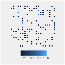
Consider m.sample, a SpatialPointsDataFrame object consisting of 100 points in {x,y} coordinate space, containing chemical results at various concentrations (“conc”). It is easily plot using spcv::convert_spdf_for_ggplot2() (also see spcv::theme_basic() for reproducing the aesthetic below).

```{r load_example} devtools::load_all() m.sample <- m3_sample head(m.sample,3)

```{r, echo = T, fig.height= 3,fig.width = 3, fig.align= "left"}
ggplot(spcv::convert_spdf_for_ggplot2(m.sample, "conc"), 
       aes(x,y, col =z)) + 
  geom_point() + 
  spcv::theme_basic() 

""

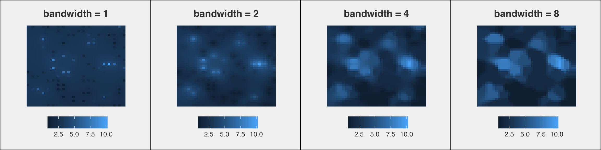
Concentrations in the study area estimated using IDW with different "bandwidths"

Use spcv() to examine interpolation errors with different bandwidths

```{r, echo = T,message = F, warning = F, results='hide'} cv.1 <- spcv(df.sp = m.sample, my_idp = 1, var_name = "conc") cv.2 <- spcv(df.sp = m.sample, my_idp = 2, var_name = "conc") cv.4 <- spcv(df.sp = m.sample, my_idp = 4, var_name = "conc") cv.8 <- spcv(df.sp = m.sample, my_idp = 8, var_name = "conc") cv.16 <- spcv(df.sp = m.sample, my_idp = 16, var_name = "conc")

![f3](https://raw.githubusercontent.com/kmayerb/spcv/master/img/f3.png)

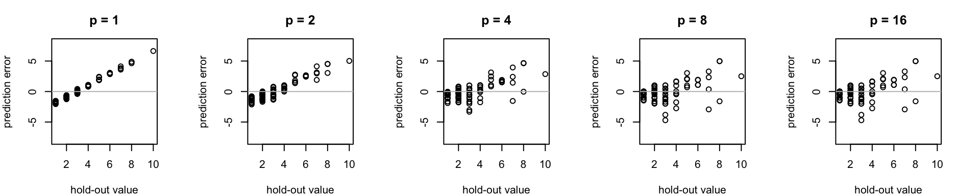
Low bandwidth (p) lends distant known points more "oomph" when interpolating unknown points. By contrast, increasing the bandwidth parameter assigns greater influence to values closer to the interpolated point. For this toy data set, the errors associated with the low-bandwidth interpolation estimate (i.e. p < 2) are similar to what would be expected using the global mean as an estimator for each unknown point. Here, medium (conc >3) and high concentration (conc > 5) samples are systematically under predicted. (error is calculated here as test value minus prediction value, so here positive sign errors repressent under prediction)

For this data, spatial cross validation illustrates how increasing the inverse distance weighting bandwidth parameter (p) reduces the magnitude of interpolation errors, but only up to a point. Which value of p is best? That probably depends on the goal of the study. For instance, for acute environmental toxins, underpredicting high concentrations may pose a larger risk than overestimating low concentrations from the standpoint of human or ecological health. 

#### Won’t you be my neighborhood?
Rather than consider the entire dataset in each IDW estimate, interpolation can be restricted to consider only points within some local neighborhood (in *gstat*, this is specified with the max distance (maxdist) argument).

#### spcv::spcv() can be used to observe the effect of tuning the neighborhood extent

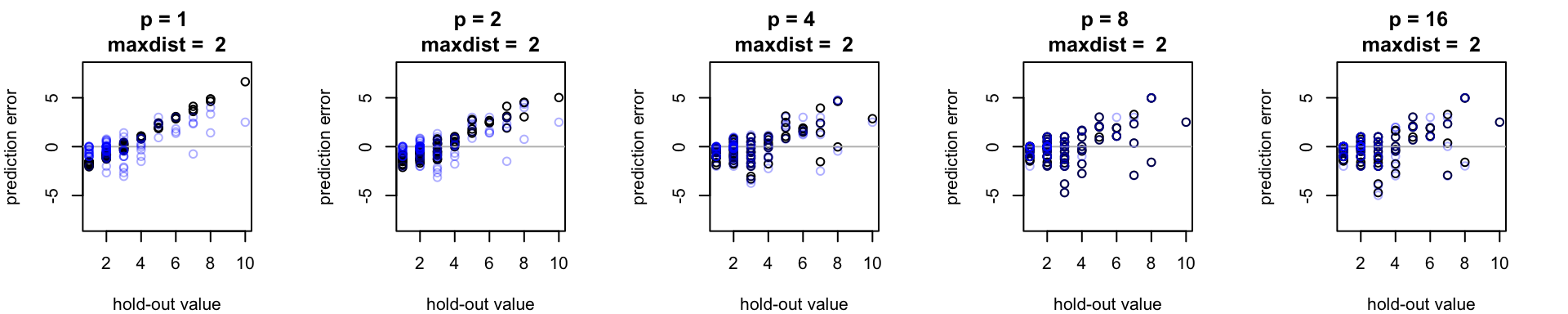
For this data set, spcv analysis shows that neighborhood extent and inverse distance weighting bandwidth (p) are related but not entirely redundant "control knobs." Visualizing the output of spcv suggests that shrinking the neighborhood extent appears to reduce the magnitude of interpolation errors for this data set, although diminishing returns kick in if higher bandwidth parameter values are selected. Nevertheless, there are clear reasons why we should consider lusing ocal over global interpolation. In particular, using a smaller local interpolation neighborhood appears to ameliorate overprediction error for lower concentration samples.

```{r neighborhood, echo = T}
my_maxdist = 2
cv.1.md  <- spcv(df.sp = m.sample, my_idp = 1, var_name = "conc", maxdist = my_maxdist)
cv.2.md  <- spcv(df.sp = m.sample, my_idp = 2, var_name = "conc", maxdist = my_maxdist)
cv.4.md  <- spcv(df.sp = m.sample, my_idp = 4, var_name = "conc", maxdist = my_maxdist)
cv.8.md  <- spcv(df.sp = m.sample, my_idp = 8, var_name = "conc", maxdist = my_maxdist)
cv.16.md <- spcv(df.sp = m.sample, my_idp = 16, var_name = "conc", maxdist = my_maxdist)

Too much of a good thing?

If things closer together in geographical space tend to be more alike, it’s tempting to push the gas on bandwidth and pump the brakes on neighborhood size (i.e., shrink the neighborhood size, while allowing all points within than neighborhood to contribute more strongly to the interpolation estimate). But eventually, the size of the data set will pose a constraint on this interpolation strategy. If we shrink the neighborhood size too much, we will be making an estimate from an extremely small sample – systematic interpolation error may or may not suffer, but I would expect this to produce highly variable interpolation errors (similare to if we had just used nearest neighbor interpolation).

One goal of the spcv package is to helps us consider this trade-off and predict, for a given data set, when our an interpolation neighborhood becomes too constrained.

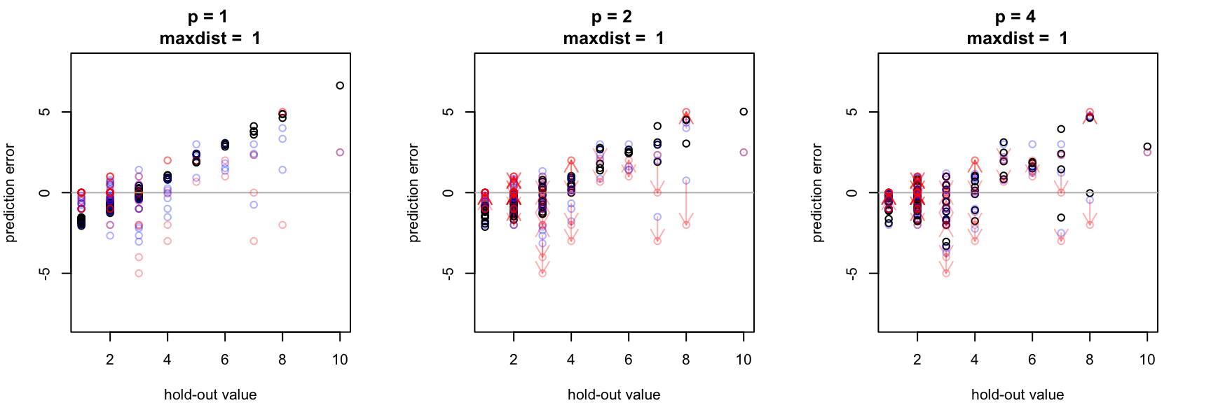
For this data set, notice how estimates in red (made with a small neighborhood size of 1 unit) seem to reduce the overall interpolation bias but also tend to lead to some larger individual errors when compared to points in blue (estimated with a larger neighborhood size).

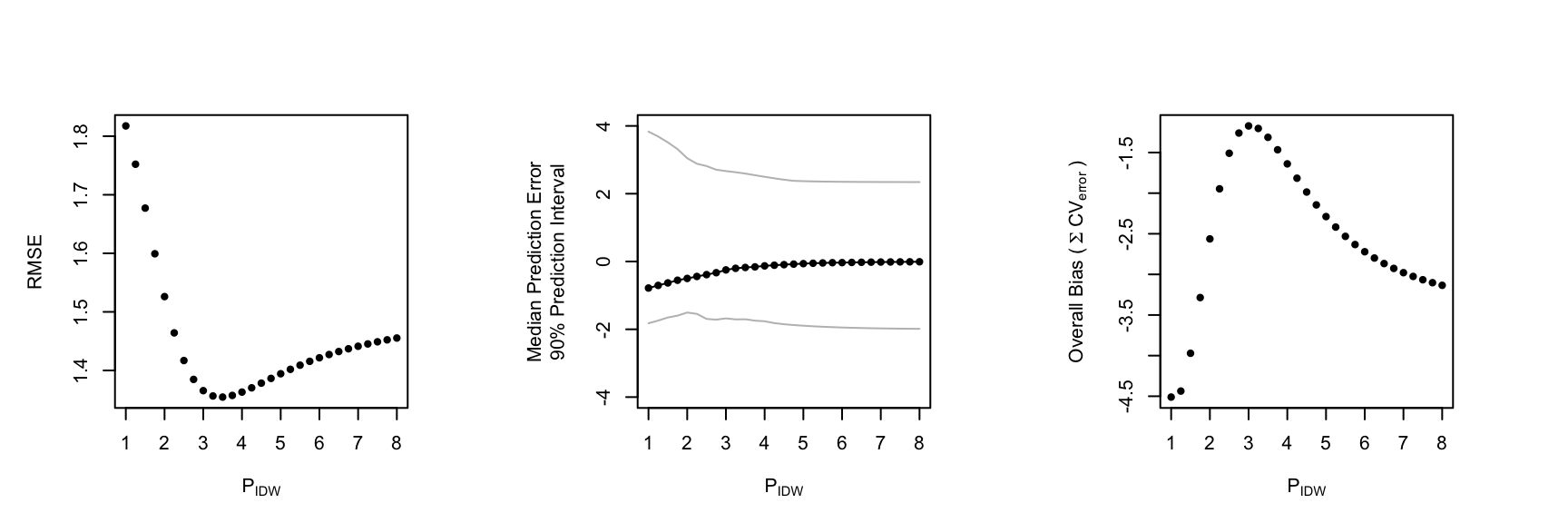
spcv as a tuning fork

To consider many possible parameterizations, spcv allows one to exploit R’s lapply function to quickly visualize cross-validation errors (i.e., a proxy for out-of-sample error) for a range of parameter values

```{r tuning fork, echo = T} cv_range = seq(1,8, by=.25) cv.t <- lapply(cv_range , function(i) spcv(df.sp = m.sample, my_idp = i, var_name = "conc"))

```

kmayerb/spcv documentation built on May 26, 2019, 2:34 a.m.