In ningzhibin/rmdocpu: Metalab report upon provided templates

htmltools::img(src = "https://raw.githubusercontent.com/ningzhibin/rmdocpu/master/inst/rmd/iMetaReport.png", 
               alt = 'logo', 
               style = 'position:absolute; top:0; right:0; padding:10px;width:100px;height:100px;')

knitr::opts_chunk$set(echo = FALSE,warning = FALSE, message = FALSE, cache = FALSE)

# enviroment setup
source("https://raw.githubusercontent.com/ningzhibin/rmdocpu/master/inst/subfunctions_general.r")
source("https://raw.githubusercontent.com/ningzhibin/rmdocpu/master/inst/subfunctions_general_update.r")

library(tidyverse)
library(ggplot2)
library(d3heatmap)
library(plotly)

# other reqruied package:
#  DT

#library(gplots)


# todo meta check

peptide.txt  <- read.delim("peptides3.txt", header = TRUE,check.names = FALSE, stringsAsFactors = FALSE)
rmarkdown::render("MQ_report_peptides_indev.Rmd", params = list(input_datatable =  peptide.txt))

rmarkdown::render("MQ_report_peptides.Rmd", params = list(input_datatable =  your_readin_tbl, meta_table = meta_table_input))

#meta_table <- read.delim("metadata.txt", header = TRUE, check.names = FALSE, stringsAsFactors = FALSE) # test with meta file

tidy_peptides <- function(peptide.txt){ 

  peptide_sequence <- peptide.txt$Sequence # only keep the first one

  # do the row wise filtering
  index_contaminant <- grep("\\+", peptide.txt$`Potential contaminant`) # note that + is a special character
  index_reverse <- grep("\\+", peptide.txt$Reverse)
  index_to_remove <- c(index_contaminant,index_reverse)

  if(length(index_to_remove) >0){ # some times there are no rows to remove
      peptide.txt <- peptide.txt[-index_to_remove,] # filtered table
      peptide_sequence <- peptide_sequence[-index_to_remove] # filtered ids
  }

  n_contaminant <- length(index_contaminant)
  n_reversed <- length(index_reverse)


  # extra the intensity column matrix
  if(any(grepl("LFQ intensity ", colnames(peptide.txt)))){ # if there are LFQ intensity columns, take out the LFQ columns
    intensity_columns <- peptide.txt[,grep("LFQ intensity ", colnames(peptide.txt))]
    colnames(intensity_columns) <- gsub("LFQ intensity ", "", colnames(intensity_columns))

  }else{ # otherwise take out intensity column, even if there is one column, without any experiment desgin

    intensity_columns <-   peptide.txt[,grep("Intensity ", colnames(peptide.txt)),drop =  FALSE]
    colnames(intensity_columns)<-gsub("Intensity ", "", colnames(intensity_columns))

  }

  return(list("intensity_matrix" = intensity_columns,
              "peptide_sequence" =peptide_sequence,
              "n_contaminant" = n_contaminant,
              "n_reversed" = n_reversed,
              "score" = peptide.txt$Score,
              "Charges" =peptide.txt$Charges,
              "length" = peptide.txt$Length,
              "misscleavage" = peptide.txt$"Missed cleavages"

              ))

}

# input

peptide.txt <- params$input_datatable


# Note: The folling analysis with meta info assumes that
# 1st columns as sample name, 2nd column as experiment name, 3rd column and after as grouping

meta_table <- params$meta_table

# tidy and process:

peptide_tidyed <- tidy_peptides(peptide.txt)

df_intensity <- peptide_tidyed$intensity_matrix
sparsity <- rowSums(df_intensity > 0) # here sparsity is number of present values
index_all_na_rows <- which(sparsity == 0)
df_intensity <- df_intensity[-index_all_na_rows,,drop = FALSE]
peptide_sequence <- peptide_tidyed$peptide_sequence[-index_all_na_rows]


# check meta_table

if( is.null(meta_table)){ 

  meta_info <- "* **No meta information provided**"

}else if (any(is.na(meta_table))){ 

  meta_info <-  "* **The meta information provided has missing values, please check again**"

}else if(!(all(as.vector(colnames(df_intensity)) %in% meta_table[,2]) && all( meta_table[,2] %in% as.vector(colnames(df_intensity))))){
  meta_info <-  "* **The experiment in meta information provided do not match the experiment names in the peptide.txt, please check again**"

}else{
 meta_info <-   c("* **Groups: **",unique(meta_table[,3]))  
}

# this figure height is for very tight figrues
figure_height <- 0.1*ncol(df_intensity)+4

Intro

This report provides some basic description of the peptide identificaiton from database search. Users can use this to quickly check the overal quality of the experiment Users can download the clean peptide quantification matrix for downstream analysis

Take-home figures

Number of contaminant: r peptide_tidyed$n_contaminant
Number of reversed: r peptide_tidyed$n_reversed
Number of qualified peptides: r nrow(peptide_tidyed$intensity_matrix)
Number of quailfied peptide without intensity information(0 intensitiy): r length(index_all_na_rows)
Number of experiment: r ncol(df_intensity)
All experiments: r colnames(df_intensity)

r meta_info

Peptide Charge States

Why charge state?

Peptide Charge distribution is a good sign of trypsin digestion and electric spray ionization.
In a typical ESI analysis of trytic digest, most of the peptides should have 2 charges, less peptides have 3 charges, because tryptic peptides have a lysine/arginie at the C-terminal, along with N-terminal contributing another charge. A possible miscleavage will contribute the third charge.
In a ESI procedure, peptides with 2 and more charges are easier to fragment and then identified by MS. However, too mnay charges will make the m/z of the peptide too small to escape the scan range, further more, it will also complicate the ms2 spectra.
if you see more peptides with charge 3 than charge 2 state,
It might indcate in-sufficient trypsin digesion, check the percentage of peptides with mis-cleavage site.
It migtht indcate the ESI is not sufficient/good enough.Check the distance between the ESI tip and MS oriface, if the ESI tip is dirty, if there is droplet occasionally.

peptide_charge <- as.data.frame(table(peptide_tidyed$Charges))
colnames(peptide_charge) = c("Charge_state", "Freq")

ggplot2::ggplot(data = peptide_charge)+
  geom_col(aes(x = Charge_state,y = Freq))+
  labs(title = "Charge Distribution", x = "Charge State",y = "Frequency") + 
  theme_bw() +
  theme(plot.title = element_text(hjust = 0.5),
        axis.text.x = element_text(angle = 90, hjust = 1),
        panel.grid = element_blank())

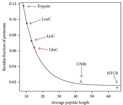
Peptide Length

Why peptide length do you expect?

Averge length of tryptic peptide is around 10.
refer to this page for peptide length. *

peptide_length <- as.data.frame(table(peptide_tidyed$length))
colnames(peptide_length) = c("peptide_length", "Freq")


ggplot2::ggplot(data = peptide_length)+
  geom_col(aes(x = peptide_length,y = Freq))+
  labs(title = "Peptide Length Distribution", x = "Peptide Length",y = "Frequency") + 
  theme_bw()+
  theme(plot.title = element_text(hjust = 0.5),
        axis.text.x = element_text(angle = 90, hjust = 1),
        panel.grid = element_blank())

Peptide Score distribution

Why peptide length do you expect?

The average score should be around 50

df_score <- data.frame(Score  = peptide_tidyed$score)


ggplot2::ggplot(data=df_score, aes(Score)) +
  geom_histogram(aes(y=..density..),color= "black",fill="white")+
  geom_density(alpha=.2, fill="#5DADE2")+
  labs(title = "Peptide Score Distribution", x = "Peptide Score",y = "Density") + 
  theme_bw()+
  theme(plot.title = element_text(hjust = 0.5),
        axis.text.x = element_text(angle = 90, hjust = 1),
        panel.grid = element_blank())

Quantification Sparsity Distrubition

In most cases, label-free quantification provides a decent way for metaproteomics profiling.

Sparsity Profile

The more peptide of 100% presence the better

df_sparsity <- as.data.frame(table(sparsity))
df_sparsity_dec <- df_sparsity[order(df_sparsity$sparsity,decreasing = TRUE),]
df_sparsity_dec$sparsity <- factor(df_sparsity_dec$sparsity, levels = df_sparsity_dec$sparsity)


ggplot2::ggplot(data = df_sparsity_dec)+
  geom_col(aes(x = sparsity,y = Freq))+
  labs(title = "Sparsity Distribution", x = "Number of Presence",y = "Frequency") + 
  theme_bw()+
  theme(plot.title = element_text(hjust = 0.5),
        axis.text.x = element_text(angle = 90, hjust = 1),
        panel.grid = element_blank())

Sparsity cummulative curve

Figure shows how many peptides have more than N presence, which helps to set the presence cutoff

#df_sparsity_dec <- df_sparsity[order(df_sparsity$sparsity,decreasing = TRUE),]

df_sparsity_dec$cumsum <-  cumsum(df_sparsity_dec$Freq)

# redefine the sparisty sequence, in order to keep the order in the plot, This is the best way as far as I know
#df_sparsity_dec$sparsity <- factor(df_sparsity_dec$sparsity, levels = df_sparsity_dec$sparsity)


ggplot2::ggplot(data = df_sparsity_dec)+
  geom_col(aes(x = sparsity,y = cumsum))+
  labs(title = "Sparsity Distribution", x = "Number of Presence",y = "Frequency") + 
  theme_bw()+
  theme(plot.title = element_text(hjust = 0.5),
        axis.text.x = element_text(angle = 90, hjust = 1),
        panel.grid = element_blank())

Peptide Intensity disitribution across samples/experiments

#note: in this log10 intenisty matrix, 0 is converted into infinity, therefore will not show in the box plot, and does not affect the distribution
df_intensity_log10 <-log10(df_intensity)

data_matrix_log10_melt<-reshape2::melt(as.matrix(df_intensity_log10))

colnames(data_matrix_log10_melt) <- c("Proteins", "Samples", "Log10(Inensity)")

ggplot(data_matrix_log10_melt)+
    geom_boxplot(aes(x = Samples, y = `Log10(Inensity)`)) +
    labs(title = "Peptide Intensity Distribution", x = "Number of Presence",y = "Frequency") + 
    theme_bw()+
    theme(plot.title = element_text(hjust = 0.5),
        axis.text.x = element_text(angle = 90, hjust = 1),
        panel.grid = element_blank())+
    coord_flip()

r if(ncol(df_intensity) > 1){ "# Overall Expression Profile"}

r if(ncol(df_intensity) > 1){ "## Heatmap"}

r if(ncol(df_intensity) > 1){"### Heatmap of Q100 peptides (with 100% presence across experiments)" }

# for files of big size, only show limited number of rows (Q100) for the test
# for interactive html display, only use top100 peptide

if(ncol(df_intensity) > 1){ # only if there are more than 1 columns in experssion matrix, we can do the heatmap and even cluster with 3 or more samples

  sparsity <- rowSums(df_intensity > 0) 
  index_Q100 <- which(sparsity == ncol(df_intensity)) # index_Q100 is the index of Q100 peptide
  df_intensity_Q100 <- df_intensity[index_Q100, , drop = FALSE] # the Q100 peptide matrix

  # plot a heatmap of Q100
  df_intensity_Q100_log10 <- log10(as.matrix(df_intensity_Q100))
  matrix_quick_heatmap(df_intensity_Q100_log10, scale = "row")
  #d3heatmap(df_intensity_Q100_log10,show_grid = FALSE) # this will slow down the rendering of the html rendering
}


# this is for the next section
if(length(index_Q100) >100){
  topN = 100
}else{
  topN = length(index_Q100)
}

r if(ncol(df_intensity) > 1){"### Heatmap of Top 100 Intensity peptides" }

  if(ncol(df_intensity) > 1){ # only if there are more than 1 columns in experssion matrix

   #heatmap of top N    # will wrap this to a function

   peptide_sequence_keep <- peptide_sequence[index_Q100] # keep the Q100 pepide sequence 
   df_intensity_Q100$peptide_total_intensity<- rowSums(df_intensity_Q100) # add total intensity column
   df_intensity_Q100$peptide_sequence <- peptide_sequence_keep # add peptide sequnce column


   df_intensity_topN <- dplyr::top_n(df_intensity_Q100, topN, peptide_total_intensity) # top 100 rows
   rownames(df_intensity_topN) <- df_intensity_topN$peptide_sequence # give the row names back


   df_intensity_topN <-df_intensity_topN[, 1: (ncol(df_intensity_topN)-2)] # delete the last 2 column
   df_intensity_topN_log10 <-log10(df_intensity_topN) # log10

    if(params$if_html){


      d3heatmap(df_intensity_topN_log10,show_grid = FALSE) # this also works

      # incorporate this figure is going to have 4M extra in file size, 
      # 
      # library(canvasXpress)
      # canvasXpress(
      #   data=t(df_intensity_topN_log10),
      #   #smpAnnot=x,
      #   #varAnnot=z,
      #   heatmapIndicatorWidth = 200, # for the color bar
      #   heatmapIndicatorHeight = 30,
      #   heatmapIndicatorHistogram = TRUE,
      # 
      #   heatmapIndicatorPosition ="topLeft",
      #   colorSpectrum=list("blue", "white", "red"),
      #   #colorSpectrumBreaks =list(8, 9,10),
      #   graphType="Heatmap",
      #   heatmapCellBoxColor="rgb(255,255,255)",
      #   samplesClustered=TRUE,
      #   showTransition=FALSE,
      #   title="Expression Profile",
      #   variablesClustered=TRUE,
      #   smpLabelScaleFontFactor=0.5,
      # 
      #   width = 800,
      #   height = 800
      # )



    }else{
      matrix_quick_heatmap(as.matrix(df_intensity_topN_log10), scale = "none")

    }
}

r if(ncol(df_intensity) > 3){"# PCA Analysis"}

if(ncol(df_intensity) > 3){ # otherwise, no point doing PCA

  #df_intensity_log10 <- log10(df_intensity+1)

  if(is.null(meta_table)){

    #pca <-PCA_wrapper_prcomp2(data_matrix = as.matrix(df_intensity_log10), inputation = TRUE)
    PCA_result <- prcomp(t(df_intensity_Q100_log10))
    loading <- as.data.frame(PCA_result$x)

  # for screen plot
    sd <- PCA_result$sde
    var <- sd^2
    var.percent <- var/sum(var) * 100

    PCs <- paste("PC", 1:length(var.percent))
    df_scree <- data.frame(PC  = factor(PCs, levels = PCs), ratio =var.percent)


    ggplot(data=df_scree, aes(x=PC, y=ratio)) + geom_bar(stat="identity")+
      labs(title = "PCA Scree Plot", x = "Component", y = "Ratio of variance") + 
      theme_bw() +
      theme(plot.title = element_text(hjust = 0.5),
      axis.text.x = element_text(angle = 90, hjust = 1),
      panel.grid = element_blank())  #+coord_flip()




    if(params$if_html){
      plot_ly(loading, x = ~PC1, y = ~PC2, z = ~PC3) %>%
      add_markers() %>%
      add_text(text = row.names(loading))

    }else{

      ggplot(loading, aes(x=PC1, y=PC2)) +geom_point(shape=1)  +
      labs(title = "PCA Plot", x = "PC1", y = "PC2") + 
      theme_bw() +
      theme(plot.title = element_text(hjust = 0.5),
      axis.text.x = element_text(angle = 90, hjust = 1),
      panel.grid = element_blank()) 

      library("scatterplot3d") # load
      scatterplot3d(loading)
    }

  }else{

    # do pca analysis with meta groupign information

    pca <-PCA_wrapper_prcomp2(data_matrix = as.matrix(df_intensity_log10), data_meta =  meta_table[,c(2,3)], inputation = FALSE)


    # plotting
    print(pca$pca_scree_plot)

      cat("Scree plot ##  shows the performance of the PCA analysis, the more percentage the top procomponets accounts, the better separation")

    print(pca$pca_component_plot)

      cat("2d PCA Component plot ##")

    print(pca$pca_confidence)

      cat("2d PCA Component plot ## with confidence boundaries")

    print(pca$pca_component_plot_kmeans)

      cat("2d PCA Component plot with K-means grouping, which is non-supervised grouping ")

    # pca$pca_component_plot_3d_interactive

  }

}

r if(length(unique(meta_table[,3])) >=2 && all(table(meta_table[,3]) >=2)) {"# ANOVA TEST \n**Peptides with significiant(p < 0.05) change between any groups**"}

# will do this block while: 1, more than (includeing) two meta/groups, 2, each group has more than (includeing) 2 samples.

if(length(unique(meta_table[,3])) >=2  && all(table(meta_table[,3]) >=2)){

pvalues_anova <- matrix_PostHoc(df_intensity,meta_table[,3])

df_intensity_p <- cbind(pvalues_anova, df_intensity)

rownames(df_intensity_p) <- peptide_sequence

df_intensity_p_filtered <- df_intensity_p[which(!is.na(df_intensity_p$p_PostHoc_pairs)),]

DT::datatable(df_intensity_p_filtered, extensions = 'Buttons',options = list(dom = "Blfrtip",scrollX=TRUE, buttons = list('copy', 'print', list(
        extend = 'collection',
        buttons = c('csv', 'excel', 'pdf'),
        text = 'Download'
      ))))

}

Download the neat table

The table is clean peptides expression table, with reversed and contaminant removed. The values are the LFQ(with label free quantification turned on) or raw protein intensity from Maxquant output. You can download/export and start from this table for downstream analysis using the (i)Metalab faminly apps.

The talbe can be further visualized by our shiny apps shiny.imetalab.ca

df_intensity <- as.data.frame(df_intensity)

rownames(df_intensity) <- peptide_sequence


# DT table is not the bottle neck for slow loading, instead, plotly figures is 
if(params$if_html){
  DT::datatable(df_intensity[1:100,], extensions = 'Buttons',options = list(dom = "Blfrtip",scrollX=TRUE, buttons = list('copy', 'print', list(
        extend = 'collection',
        buttons = c('csv', 'excel', 'pdf'),
        text = 'Download'
      ))))

}else{
  knitr::kable(df_intensity[1:100,])
}