In r-tmap/tmap: Thematic Maps

knitr::opts_chunk$set(
  collapse = TRUE,
  out.width = "100%",
  dpi = 300,
  fig.width = 7.2916667,
  comment = "#>"
)
hook_output <- knitr::knit_hooks$get("output")
knitr::knit_hooks$set(output = function(x, options) {
   lines <- options$output.lines
   if (is.null(lines)) {
     return(hook_output(x, options))  # pass to default hook
   }
   x <- unlist(strsplit(x, "\n"))
   more <- "..."
   if (length(lines)==1) {        # first n lines
     if (length(x) > lines) {
       # truncate the output, but add ....
       x <- c(head(x, lines), more)
     }
   } else {
     x <- c(more, x[lines], more)
   }
   # paste these lines together
   x <- paste(c(x, ""), collapse = "\n")
   hook_output(x, options)
 })

library(tmap)
tmap_options(scale = 2) # to make high-res screenshots
# for the screenshots, height was set to 1200

Shiny integration

library(shiny)

Three functions take care of integrating tmap maps in shiny: tmapOutput(), renderTmap(), and tmapProxy()

Plot mode

An (almost) minimal example of a choropleth where the data variable is selected via a select input widget:

NLD_vars <- setdiff(names(NLD_dist), c("code", "name"))
tmap_mode("plot")
shinyApp(
  ui = fluidPage(
    tmapOutput("map", height = "1000px"),
    selectInput("var", "Variable", NLD_vars)
  ),
  server <- function(input, output, session) {
    output$map <- renderTmap({
      tm_shape(NLD_dist) +
        tm_polygons(input$var, zindex = 401, lwd = 0.5) +
      tm_shape(NLD_muni) +
        tm_borders(lwd = 1, col = "black") +
      tm_shape(NLD_prov) +
        tm_borders(lwd = 2, col = "black") +
      tm_layout(meta.margins = c(0, 0, 0, 0.15)) # fixed margin for the legend
    })
  }, 
  options = list(launch.browser = TRUE)
)

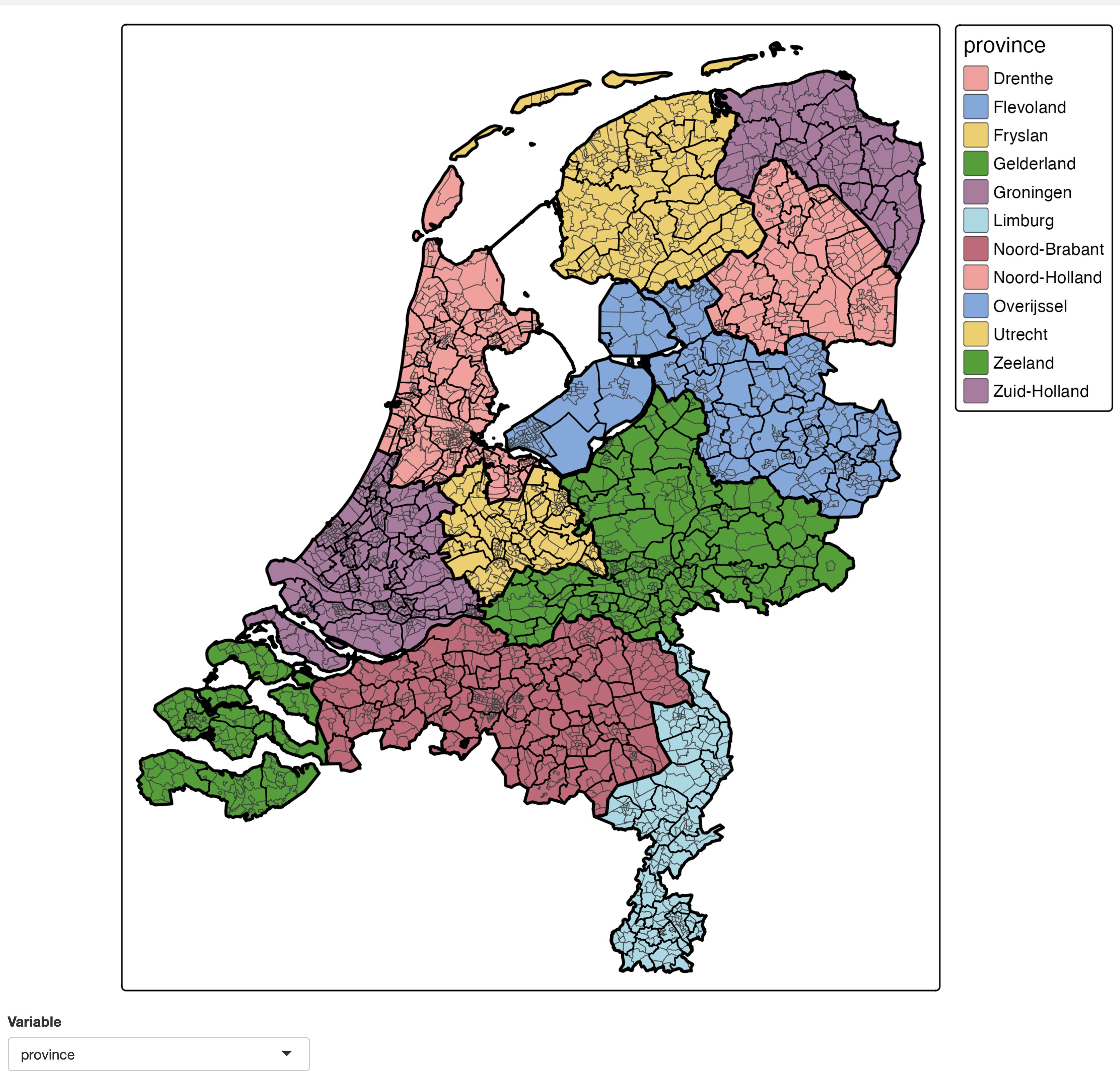
Note that setting meta.margins in the last tmap line is needed to make sure the map stays in the same position after rendering. Without this line (so by default) the horizontal position of the map depends on the legend width, which in turn depends on the legend title /item labels.

Also note that because the map is redrawn every time the inputs change, proxy objects via tmapProxy() cannot be used. The are used in "view" mode as well see next.

View mode

tmap_mode("view")

When inputs are changed in "view" mode, it is preferable that the focus (zoom and panning location) does not change. That is where tmapProxy() comes into play. It updates the mape. Old layer are removed via tm_remove_layer() and new layer can be added.

It is recommended to:

• Set zindex for each map layer, because this determines the plotting order (which is not necessarily the order of call anymore, because of these removals and additions).
• To use basemaps, transform spatial vector data to sf objects in the crs (EPSG) 4326 and spatial raster data to stars objects in the crs (EPSG) 3857. Why? Because these operations take time, albeit less than a second. If you let tmap do this job, it happens every time the map is updated. In an interactive session, every millisecond counts. Therefore it is advisable to do this as one-time operation before using tmap.

library(sf)
NLD_dist_4326 = st_transform(NLD_dist, 4326)
NLD_muni_4326 = st_transform(NLD_muni, 4326)
NLD_prov_4326 = st_transform(NLD_prov, 4326)

shinyApp(
  ui = fluidPage(
    tmapOutput("map", height = "1000px"),
    selectInput("var", "Variable", NLD_vars)
),
server <- function(input, output, session) {
  output$map <- renderTmap({
    tm = tm_shape(NLD_dist_4326) +
      tm_polygons(
        fill = NLD_vars[1], 
        fill.scale = tm_scale(style = "kmeans", values = "matplotlib.plasma"),
        id = "code", zindex = 401, lwd = 0.5) +
      tm_shape(NLD_muni_4326) +
        tm_borders(lwd = 1, col = "black", zindex = 402) +
      tm_shape(NLD_prov_4326) +
        tm_borders(lwd = 2.5, col = "black", zindex = 403) +
      tm_layout(meta.margins = c(0, 0, 0, 0.3))  # fixed margin for the legend
  })
  observe({
    var <- input$var
    tmapProxy("map", session, {
      tm_remove_layer(401) + 
      tm_shape(NLD_dist_4326) +
        tm_polygons(input$var, 
          fill.scale = tm_scale(style = "kmeans", values = "matplotlib.plasma"),
          id = "code", zindex = 401, lwd = 1)
    })
  })
}, 
options = list(launch.browser = TRUE)
)

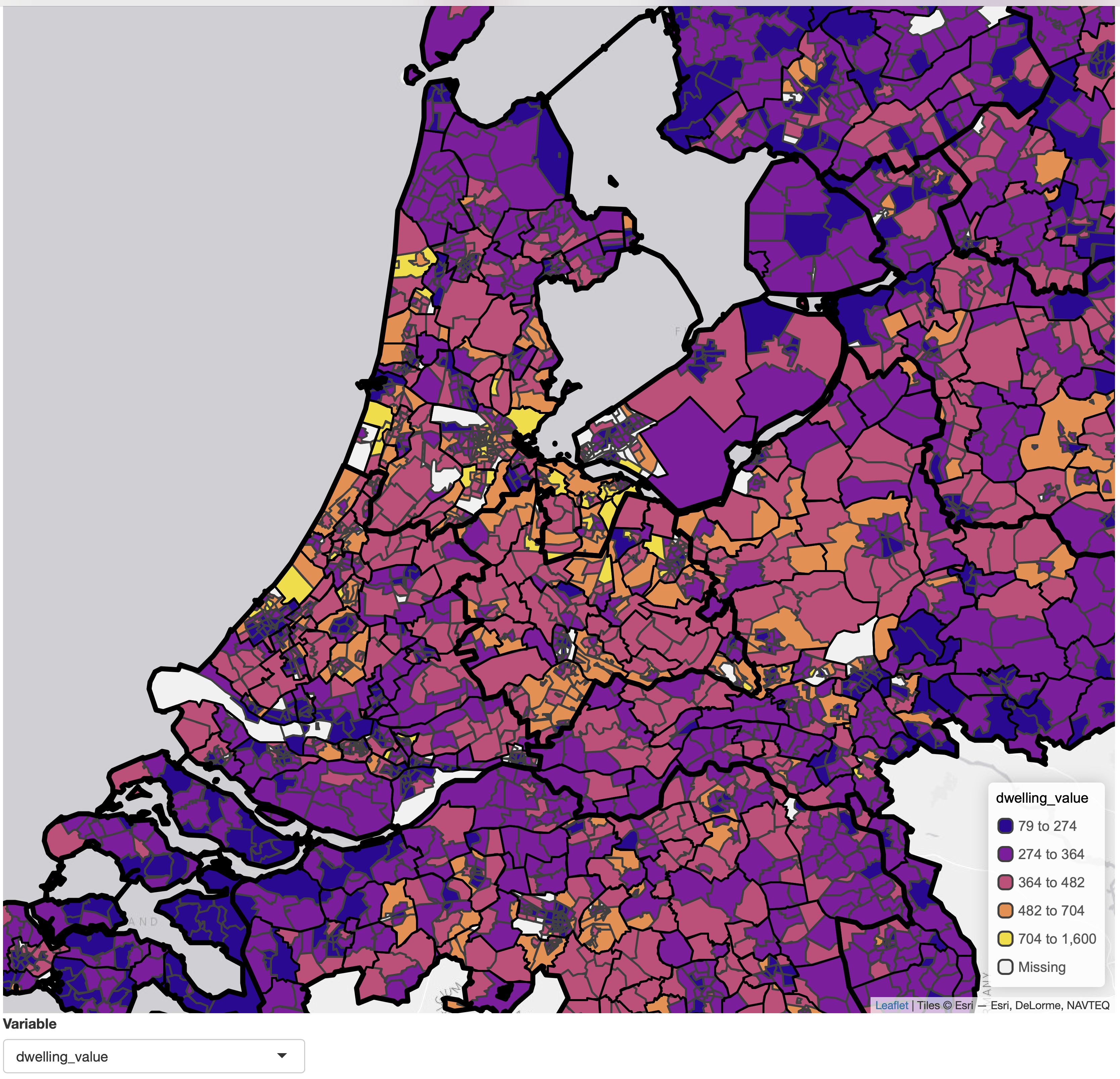Note that we improved the scale that we applied for each variable. Because most data variables are numeric, and because most of them are skewed (e.g. dwelling value), we've used the general purpose function tm_scale() to set the class interval to kmeans and the color palette to "matplotlib.plasma". Run cols4all::c4a_gui() to explore color palettes.

r-tmap/tmap documentation built on Feb. 28, 2025, 7:54 a.m.