In ropensci/gtfsr: Working with GTFS (General Transit Feed Specification) feeds in R

knitr::opts_chunk$set(collapse = TRUE, cache=FALSE, comment = "#>", fig.width=7.3, fig.height=5)

gtfsr (v1.0.3)

gtfsr is an R package for easily importing, validating, and mapping transit data that follows the General Transit Feed Specification (GTFS) format.

The gtfsr package provides functions for converting files following the GTFS format into a single gtfs data objects. A gtfs object can then be validated for proper data formatting (i.e. if the source data is properly structured and formatted as a GTFS feed) or have any spatial data for stops and routes mapped using leaflet. The gtfsr package also provides API wrappers for the popular public GTFS feed sharing site TransitFeeds, allowing users quick, easy access to hundreds of GTFS feeds from within R.

1. Get an GTFS API key

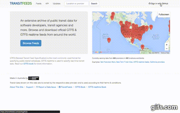
This package can get data from a user-specified URL and is also able to get GTFS data from the TransitFeeds API. This vignette will focus on the case where GTFS data is extracted from the TransitFeed API. Below are the steps needed to get a API key (note: requires a GitHub account), including a YouTube (click the GIF to see the YouTube video) that visually guides you through the steps.

1. Go to http://transitfeeds.com/
2. Click "Sign in with GitHub" in the top-right corner.
   • If it is your first time visiting the site, it will ask you to sign in (and likely every time if you do not have cookies enabled).
3. Once signed in, click your profile icon in the top-right and select "API Keys" from the drop-down menu.
   • Your GitHub profile icon and username replaces "Sign in with GitHub".
4. Fill in "Enter a description" and then click the "Create Key" button.
5. Copy your new API Key to your clipboard.

2. Use gtfsr package to download feed list

First things first, load the gtfsr package and set your key to access the TransitFeeds API. This example also using the dplyr package to manage data frames and magrittr for piping.

library(gtfsr)
library(dplyr)
options(dplyr.width = Inf) # I like to see all the columns
library(magrittr)

# set_api_key() # input your API key here

Getting full list of available GTFS feeds

With a valid API key loaded, you can easily get the full list of GTFS feeds using the get_feedlist function. What we care most about are the feed GTFS data urls contained in column url_d of the feed list. Since we are interested in acquiring the GTFS data (not just the feedlist), we can use the filter_feedlist() function to return a data frame containing only valid feed urls.

By default, filter_feedlist() only checks to make sure each links starts with http[s]://. To check the link is actually working, use option test_url = TRUE. But beware, this can take a while!

feedlist_df <- readRDS(here::here("data-raw/feedlist_df"))
gtfs_obj    <- readRDS(here::here("data-raw/gtfs_obj"))

feedlist_df <- get_feedlist() # create a data frame of all feeds

feedlist_df <- feedlist_df %>% filter_feedlist() # filter the feedlist

feedlist_df %>% select(url_d) %>% head(5) # show first 5 feed urls

Here is a map of all available locations.

leaflet::leaflet() %>% leaflet::addTiles() %>%
    leaflet::addCircleMarkers(data = feedlist_df, lat = ~loc_lat, lng = ~loc_lng, popup = ~paste(sep = "<br/>", t, loc_t))

Subsetting the GTFS feedlist

If we want only the data for a specific location (or locations), we can get then search the feedlist for feeds of interest.

Assume we are interested in getting all the GTFS data from Australian feeds (i.e. we search for location names for the word 'australia'). We can match Australian agencies by name (filter on loc_t) and extract the corresponding url feeds (select url_d).

## get australian feeds
aussie_df <- feedlist_df %>%
    filter(grepl('australia', loc_t, ignore.case = TRUE)) # filter out locations with "australia" in name

aussie_df %>% select(loc_t) %>% head(5) # look at location names

aussie_urls <- aussie_df %>% select(url_d) # get aussie urls

Once we have the urls for the feeds of interest, we can download and extract all the GTFS data into a list of gtfs objects using the import_gtfs function.

gtfs_objs <- aussie_urls %>% slice(c(6,9)) %>% import_gtfs()

Inspecting Parsing Errors/Warnings

During the import of the any feed url, you will see the following message:

NOTE: Parsing errors and warnings while importing data can be extracted from any given data frame with `attr(df, "problems")`.

This output was suppressed in the last section to save space given how verbose it is. But the highlighted NOTE explains that if one observes an error or warning during the import process, one can extract a data frame of problems, which is stored as an attribute for any data frame contained within any gtfs object that had a warning output.

As an example, let's extract the gtfs data and problems data for a url with parsing errors/warnings. You can use import gtfs without going through transitfeeds.com if you choose too.

url <- 'http://www.co.fairbanks.ak.us/transportation/MACSDocuments/GTFS.zip'

gtfs_obj <- url %>% import_gtfs()

If you look at the console output when creating the gtfs_obj object, you could see this kind of warning.

...
Reading calendar.txt
Warning: 2 parsing failures.
row col   expected    actual
  3  -- 10 columns 1 columns
  4  -- 10 columns 1 columns
...

To understand the problem, let's extract the data frame calendar_df. Recall that import_gtfs returns either a single gtfs list object (if one url is provided) or a list of gtfs objects.

# extract `calendar_df` from gtfs_obj
df <- gtfs_obj$calendar_df

df

attr(df, 'problems')

From inspecting the output from attr(df, 'problems') and comparing it to df, it appears the problems for this particular calendar_df stem from the empty rows added to the end of the original text file. Not a big deal and easily cleaned to fit the standard but we leave such specific fixes to the user to correct.

3. Mapping networks, routes, and stops using gtfsr

The gtfsr has mapping functions designed to help users quickly map spatial data that is found within most GTFS feeds. These functions input gtfs objects and then map the desired datum or data (stop, route, route networks).

There are two mapping functions:

1. map_gtfs is flexible function used for mapping route shapes and stops. Once can specify the agency (there can be more than one per feed) and/or specific routes by route ID.
2. map_gtfs_stop is a simple function used for mapping a single stop.

Example: Duke University

Let's investigate Duke University's transit system.

First, we convert its GTFS transit feed into a gtfs object.

duke_gtfs_obj <- feedlist_df %>%
    filter(grepl('duke', t, ignore.case=TRUE) & # note, we search `t` (agency name)
           grepl('NC, USA', loc_t, ignore.case=TRUE)) %>%  # get NC agencies
    select(url_d) %>%   # get duke university feed url
    import_gtfs(quiet=TRUE)     # suppress import messages and prints

Mapping an agency route network

We can get visualize all of the routes that make up Duke University's Transit system using map_gtfs and just passing the gtfs objected duke_gtfs_obj. This is because the Duke University Transit system is made of only one agency (duke_agency_name = "Duke Transit") and, when you pass a single gtfs object, the default behavior of map_gtfs is to take the first observed agency name and plot all it's routes.

map_gtfs(gtfs_obj = duke_gtfs_obj) # map all routes of agency with stops

# below is equivalent because duke only has a single agency.
duke_agency_name <- duke_gtfs_obj[['agency_df']]$agency_name[1]
map_gtfs(gtfs_obj = duke_gtfs_obj, agency_name = duke_agency_name)

If desired, we can also omit stops for every route in the network by using option include_stops = FALSE (this option is include_stops = TRUE by default).

duke_agency_name <- duke_gtfs_obj[['agency_df']]$agency_name[1]
map_gtfs(gtfs_obj = duke_gtfs_obj, agency_name = duke_agency_name, include_stops = FALSE) # map all routes of agency, with no stops

Mapping routes and route stops

Let's get more specific and map out all stops and the shape of the popular C1 East-West Loop bus route. We need only find the route_id before mapping all the stops using map_gtfs(..., only_stops = TRUE) and the shape using map_gtfs(..., only_stops = FALSE).

C1_route_id <- duke_gtfs_obj[['routes_df']] %>%
    slice(which(grepl('C1', route_short_name, ignore.case=TRUE))) %>% # search for "C1"
    extract2('route_id') # extract just the datum in route_id

map_gtfs(gtfs_obj = duke_gtfs_obj, route_ids = C1_route_id) # map route shape with stops, the default
map_gtfs(gtfs_obj = duke_gtfs_obj, route_ids = C1_route_id, include_stops = FALSE) # map just the route shape, no stops
map_gtfs(gtfs_obj = duke_gtfs_obj, route_ids = C1_route_id, only_stops = TRUE) # map all stops along route using `only_stops = TRUE`

We can also map more than one route shape at a time by passing 2 or more route IDs. Let's add the Central Campus Express CCX. (Note this feature does not exists for route stops but it's coming soon.)

C1_CCX_route_ids <- duke_gtfs_obj[['routes_df']] %>%
    slice(which(grepl('C1|CCX', route_short_name, ignore.case=TRUE))) %>% # search for "C1"
    extract2('route_id') # extract just the datum in route_id

map_gtfs(gtfs_obj = duke_gtfs_obj, route_ids = C1_CCX_route_ids) # pass multiple route IDS and map route shapes with stops (the default)

Mapping a single stop

Sometimes, one wants to see a single stop. For example, the C1 idles at one of the busiest stops at Duke---the "West Campus Chapel" stop. (This bus stop is located in front of Duke University's iconic gothic Chapel, Duke's most famous landmark.) Let's isolate this stop and map it.

We can search the required field stop_name for something that matches "West Campus Chapel" with a combination of dplyr::slice plus which and grepl.

# look for west chapel stop
west_chapel_stop_id <- duke_gtfs_obj[['stops_df']] %>%
    slice(which(grepl('west campus chapel', stop_name, ignore.case=TRUE))) %>%
    extract2('stop_id') # extract just the stop_id

west_chapel_stop_id

Now, we can map the stop using the function map_gtfs_stop().

map_gtfs_stop(gtfs_obj = duke_gtfs_obj, stop_id = west_chapel_stop_id, stop_color = 'blue')

4. Validating the file and fields structure of a GTFS feed

GTFS feeds contain required and optional files. And within each of these files, there are also required and optional fields (For more detailed information, please see Google's GTFS Feed Specification Reference. Information on non-standard GTFS files---specifically timetables-new.txt and timetable_stop_order-new.txt---can be found at the GTFS-to-HTML repo.

After one has successfully downloaded and unpacked a transit feed, there is no guarantee that it satisfies the requirements of a valid GTFS feed. For example, an unpacked directory may contain all the properly named text files (e.g. agency.txt, stops.txt, etc), but it could be that within each text file there is no data or that some of the required fields (or variables) (e.g. stop_id) are missing.

The gtfsr package can quickly check the file and field structure of a GTFS feed and inform you if all required files and fields have been found. Additional information about optional files and fields is also provided. The function is called validate_gtfs_structure(). It inputs an object of class gtfs (the output of functions import_gtfs() or read_gtfs()) and by default, attaches the validate attribute (i.e. attr(gtfs_obj, 'validate')) to the gtfs object. The validate attribute is just a list of validation information. Set the option return_gtfs_obj = FALSE if you only want this validation list.

Let's take a look at an example, using transit feed data from agencies in Durham, NC, USA.

nc <- feedlist_df %>%
    filter(grepl('NC, USA', loc_t, ignore.case=TRUE)) # get NC agencies

durham_urls <- nc %>%
    filter(grepl('durham', loc_t, ignore.case=TRUE)) %>%
    select(url_d) # get durham urls

gtfs_objs <- durham_urls %>% import_gtfs(quiet=TRUE) # quietly import

sapply(gtfs_objs, class) # verify that each object of is a `gtfs` object

# validate file and field structures ----------
# attach `validate` data as attribute
gtfs_objs_w_validate <- lapply(gtfs_objs, validate_gtfs_structure)

# extract `validate` attribute data
validate_list_attr <- lapply(gtfs_objs_w_validate, attr, which = 'validate')

# extract validation data directly
validate_list_direct <- lapply(gtfs_objs, validate_gtfs_structure, return_gtfs_obj = FALSE)

# both methods work. option `return_gtfs_obj = FALSE` is more direct
identical(validate_list_attr, validate_list_direct)

The validate attribute (or list) will always contain 4 elements:

• all_req_files a logical value which checks if all required files have been found
• all_req_fields_in_req_files a logical value which checks if all required fields within required files have been found
• all_req_fields_in_opt_files a logical value which checks if all required fields within any optional files have been found (i.e. FALSE if an optional file is provided but is missing a required field)
• validate_df a data frame containing all files and fields found plus their status

There can also be 3 other elements:

• problem_req_files a data frame which highlights problematic required files (required files that are either missing or have missing required fields)
• problem_opt_files a data frame which highlights problematic optional files (optional files that are missing required fields)
• extra_files a data frame of any extra files found (i.e. non-standard GTFS feed files not listed as optional or required)

Taking a closer look, we can see that not all Durham agencies provide all required files. The second object, gtfs_objs[[2]], is NULL given that the link doesn't connect to a valid feed. (The link connects you to Go Transit NC's Developer Resources page but not directly to any feeds.)

The two valid gtfs objects, gtfs_objs[[1]] and gtfs_objs[[3]], contain all required fields. However, these agencies provided optional files that are missing required fields.

validate_list_attr %>% sapply(. %>% extract2('all_req_files'))
validate_list_attr %>% sapply(. %>% extract2('all_req_fields_in_req_files'))
validate_list_attr %>% sapply(. %>% extract2('all_req_fields_in_opt_files'))

# OR, without piping
# sapply(validate_list_attr, '[[', 'all_req_files')
# sapply(validate_list_attr, '[[', 'all_req_fields_in_req_files')
# sapply(validate_list_attr, '[[', 'all_req_fields_in_opt_files')

We can get more detail about the problematic optional files by extracting the element problem_opt_fields.

# extract the `problem_opt_files` from the validation list
validate_list_attr[[3]]$problem_opt_files

We can see that the optional frequencies.txt file was provided but all of the required fields were empty.

It is important to recall that GTFS feed files and fields can contain optional fields. Therefore, while it is useful to know any potential problems with optional files provided by a given feed, we can still proceed with interesting analyses as long as we have all the required files and fields.

ropensci/gtfsr documentation built on June 11, 2022, 11:22 a.m.