In skranz/RTutor: Interactive R problem sets with automatic testing of solutions and automatic hints

---

title: Problem Set VisualMode output: html_document: keep_md: yes toc: yes

---

# Load libraries and source extra code
library(dplyr)
library(RTutor)


# Options for rendering data frames
# If you knit to a Word docx file, try
# 
# data.frame.theme="word" 
# 
# (needs RStudio > 1.2.1)
# 
# You can also set the options like
# table.max.cols as chunk options
# Makes sense if there are too many, too wide
# columns in some chunks

RTutor::set.knit.print.opts(data.frame.theme="code", table.max.rows=25, table.max.cols=NULL, round.digits=5, signif.digits=8)


# continue knitting even if there is an error
knitr::opts_chunk$set(error = TRUE) 

Exercise 1

This problem set is designed to be solved in RStudio's new Visual Mode. The solution file should be kept in the default source mode, since some RTutor syntax, like the start of a block with #< will be rewritten in visual mode. In the visual mode, HTML links, images and Latex fomulas will be nicely displayed. Let us look at an example...

Consider the following simulated code:

n = 1000
eps = rnorm(n,0,1)
x2 = rnorm(n,0,1)
x1 = rnorm(n,0,1) +x2
beta0 = 100; beta1 = 0; beta2 = 1;
y = beta0+beta1*x1+beta2*x2+eps

Estimate the following short regression:

$$y = \beta_0 + \beta_1 x_1 + u$$

# # Complete the code
# lm(___)

lm(y~x1)

---

Award: Your first regression

Great, you have run your first regression...

---

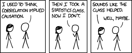
What do we learn?

(Source: xkcd)

skranz/RTutor documentation built on Feb. 7, 2024, 12:53 a.m.